Understanding root-mean-square voltage

And how do we derive its value for sine waves?

Regular readers know that I try not to assume prior knowledge of calculus in my articles on electronics. I think that even among geeks, relatively few folks are fluent in it. Many college calculus classes are a rapid-fire of poorly-explained formulas that take a long time to memorize — and only a moment to forget. Sometimes, the route is unavoidable; but most of the time, EE articles lean on it for no reason at all.

Today, I’d like to take an angry swipe at the derivation of the formula for the root-mean-square voltage (Vrms) that is currently the #1 hit on Google:

I think we can do better than that.

Hol’ up, what’s root-mean-square voltage?

This section assumes familiarity with voltage and resistance. If you need a refresher, review this article first.

Every now and then, we want to figure out the power that’s dissipated when we supply a voltage-based signal to a known resistance. A good example is sizing the amplifier circuitry for driving an audio speaker. Modern solid-state amplifiers generally deal with voltages. Speaker coils have a specified resistance and a power limit expressed in watts.

In the article linked above, we derived the following formula:

\(P = { V^2 \over R}\)

This equation makes sense if the voltage is constant — but what if the signal changes over time?

To answer that question, let’s study a toy example of a 10 Ω load and a supply voltage that changes in three discrete steps of equal duration: 1 V, 10 V, back to 1 V. In this setup, each time slice is essentially its own “steady state” scenario, so we can split the calculations accordingly:

\(\begin{array}{|l|l|} \hline \textbf{Time} & \textbf{Voltage} & \textbf{Power delivered to 10 Ω} \\ \hline t = 0 & V_0 = \textrm{1 V} & P_{0} = (\textrm{1 V})^2 / (\textrm{10 Ω}) = \textrm{0.1 W} \\ t = 1 & V_1 = \textrm{10 V} & P_1 = (\textrm{10 V})^2 / (\textrm{10 Ω}) = \textrm{10 W} \\ t = 2 & V_2 = \textrm{1 V} & P_2 = (\textrm{1 V})^2 / (\textrm{10 Ω}) = \textrm{0.1 W} \\ \hline \end{array}\)

With this done, we can compute a simple arithmetic mean to get the average power dissipated by the load over time:

\(P_{avg} = {P_0 \ +\ P_1 \ +\ P_2 \over 3} = {(0.1 \textrm{ W} \ +\ 10 \textrm{ W} \ +\ 0.1 \textrm{ W}) \over 3} = 3.4 \textrm{ W}\)

The result is correct, but this method of calculating the value is not always convenient. For example, a typical song consists of around 5 million audio samples; we can calculate the power associated with each sample, but then we’d need to redo the entire calculation to figure out the result for a different position of the volume knob. It would be better to find a single, synthetic DC voltage that works out to the same amount of power dissipation as the AC waveform. Equipped with this, we could model the effects of attenuating or amplifying the signal with more ease.

But how do we calculate that equivalent voltage? Is it just an arithmetic mean of the voltages in each time slice? Let’s continue with our three-voltage scenario and see if the numbers work out:

\(\begin{array}{c} V_{avg} = {V_0 \ +\ V_1 \ +\ V_2 \over 3} = {1 \textrm{ V} \ +\ 10 \textrm{ V} \ + \ 1 \textrm{ V} \over 3} = 4 \textrm{ V} \\ P = {(4 \textrm{ V})^2 \over 10 \textrm{ Ω}} = \xcancel{1.6 \textrm{ W}} \textrm{ - nope! } \end{array}\)

The results don’t match. The problem is the V² term in the power equation: the square of a sum is not the same as the sum of squares. To refine the approach, we can just solve the power equation for our toy example symbolically.

The component equations are P₀ = V₀ / R, P₁ = V₁ / R, and P₃ = V₃ / R, so:

\(P_{avg} = {P_0 \ +\ P_1 \ +\ P_2 \over 3} = {{V_0}^2 \ +\ {V_1}^2 \ +\ {V_2}^2 \over 3R} \)

Upon closer inspection, we can restate the result as:

\(P_{avg} = {{V_0}^2 \ +\ {V_1}^2 \ +\ {V_2}^2 \over 3} \bigg/ R \)

The first half of the expression is just an arithmetic mean of the squares of voltages, sitting right where the V² part of the constant-voltage formula used to be. Another way to put this is that we’re squaring the original waveform first, and then calculating a standard arithmetic mean of that.

Anyway, let’s call that weird mean x and confirm that the math checks out:

\(\begin{array}{c} x = {(1 \textrm{ V})^2 \ + \ (10 \textrm{ V})^2 \ +\ (1 \textrm{ V})^2 \over 3} = 34 \textrm{ V}^2 \\ P = {x \over R} = {34 \textrm{ V}^2 \over 10 \textrm{ Ω}} = 3.4 \textrm{ W} \textrm{ - correct!} \end{array} \)

But what is x in physical terms? It’s not a substitute for voltage in the original power expression; remember that it took place of the square of voltage (V²). To get the power-equivalent voltage we talked about, we need to calculate a square root of this value.

And that’s what “root mean square” voltage (Vrms) is: it’s the square root (R) of the arithmetic mean (M) of the squared waveform (S). In this case, Vrms = √34 ≈ 5.831 V. We can model the effect that halving the amplitude of the input signal would have on the dissipated power simply by dividing Vrms by two.

The more practical case of a square wave that alternates between two voltages — Vlo and Vhi — is analogous to the approach discussed earlier in this section, except that we only need to calculate the mean of two points instead of three:

\(V_{rms} = \sqrt{{V_{lo}}^2 + {V_{hi}}^2 \over 2}\)

But what about signals that change in a continuous way?

Vrms for sine waves

In analog electronics, we often work with sine signals — and that’s where Wikipedia usually hits you with calculus. Can we avoid this?

The answer is yes! As a reminder, to find the RMS of an arbitrary waveform, we need to calculate the square root (R) of the arithmetic mean (M) of the squared waveform (S).

We can start by squaring the waveform. The general equation for a sine wave signal of a given peak amplitude Vp is as follows:

\(V(t) = V_{p} \cdot sin(2 \pi f t)\)

Squaring the right-hand side yields:

\([V_p \cdot sin(2 \pi f t) ]^2 = {V_p}^{2} \cdot sin^2(2 \pi f t)\)

The only part of the expression that changes over time is the sin²(…) function. Let’s use a new symbol — Sm — to represent its mean. This allows us to write the Vrms expression the following way:

\(V_{rms} = \sqrt{{V_p}^2 \cdot Sm} = V_p \cdot \sqrt{Sm}\)

Now, all we have to do is find Sm. To find the mean of any periodic waveform, we only need to consider a single cycle; the average of any repeated sequence is the same as the average of the basic repeating unit:

\({{1 + 2 + 3} \over 3} = {{(1 + 2 + 3) + (1 + 2 + 3) + (1 + 2 + 3)} \over 9}\)

The period of sin²(...) can’t be longer than the period of the sine function before squaring; in other words, we can safely limit ourselves to parameters between between 0° and 360°. But this still means we have an infinity of continuously-changing values to average!

Luckily, trigonometry comes to the rescue. Let’s step away from the specific Vrms scenario and consider an ad-hoc right-angled triangle described by the usual trigonometric functions:

Triangle life.

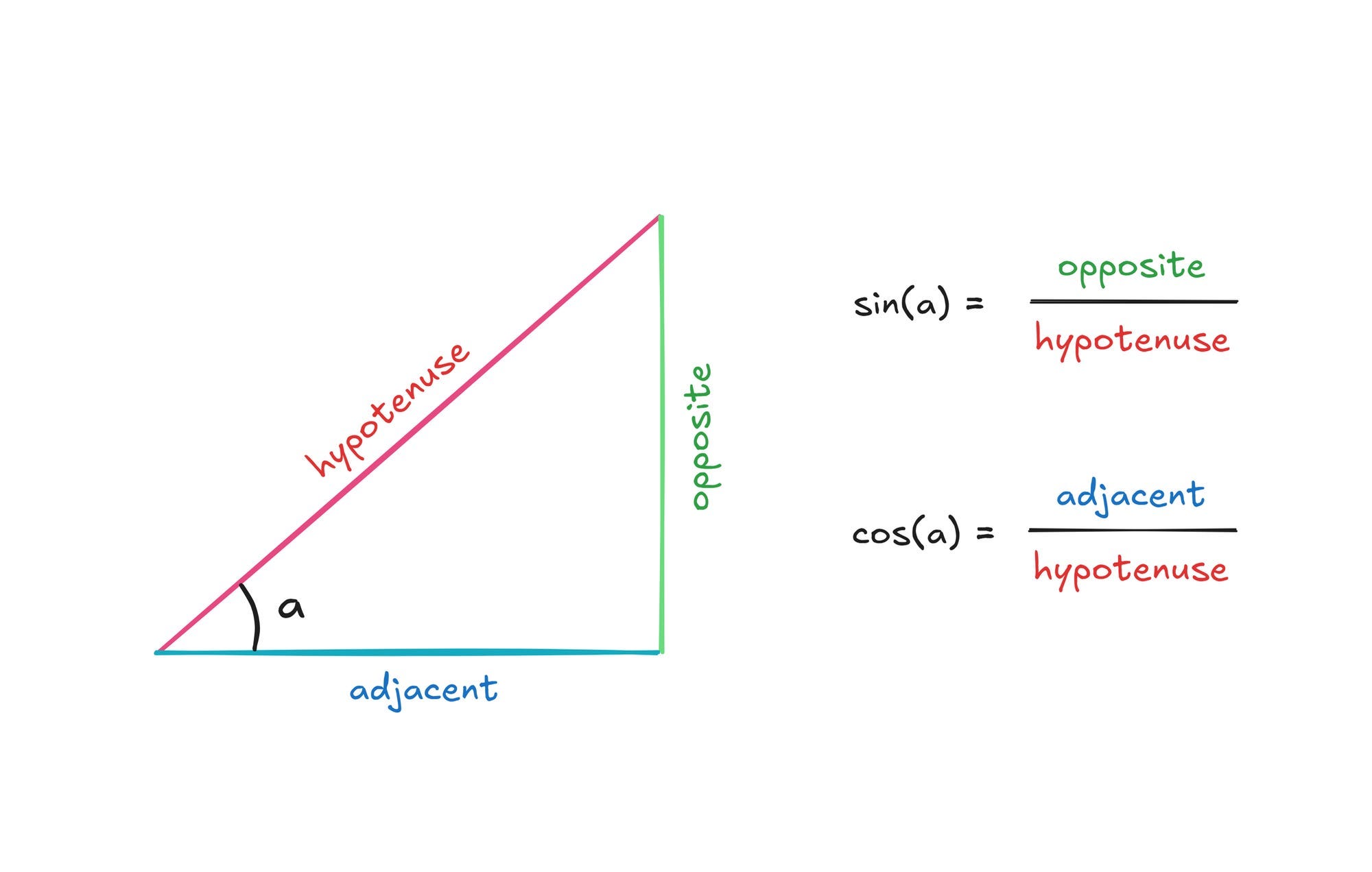
Let’s say that we know the length of the hypotenuse - call it n — and know the angle a. It should be clear that the height of the vertical edge is equal to sin(a) × n and the length of the horizontal edge is cos(a) × n.

This being a right triangle, we can also describe the relationship between its sides using the Pythagorean theorem:

\(\textrm{hypotenuse}^2 = \textrm{opposite}^2 + \textrm{adjacent}^2\)

As it happens, we already know the values for these; the hypotenuse is n an the other sides are given by the trigonometric functions of angle a. Let’s plug this in and see what comes out:

\(\begin{array}{c} n^2 = [n \cdot sin(a)]^2 + [n \cdot cos(a)]^2 \\ n^2 = {n}^2 \cdot sin^2(a) + n^2 \cdot cos^2(a) \\ \\ \textrm{...simplified:} \\ 1 = sin^2(a) + cos^2(a) \end{array} \)

This universal rule — a surprising relationship between the squares of sine and cosine — is called the Pythagorean identity.

Now, let’s circle back to the RMS conundrum. To explain the next step, imagine that you only put $5 bills in a piggy bank; it follows that the average value of the bills in the piggy bank is necessarily $5. In other words, the constraint placed on the constituent values carries over to the arithmetic mean. In the same vein, if for every given a, the value of sin²(a) + cos²(a) is equal to 1, then the average value of sums across any range of α must also be 1.

\({\overbrace{[sin^2(a_1) + cos^2(a_1)]}^{=\ 1} + ... + \overbrace{[sin^2(a_n) + cos^2(a_n)]}^{= \ 1} \over n } = 1\)

As a matter of basic arithmetic, any long fraction representing the mean can be split into two shorter fractions that group the elements any way we please:

\({{(a_1 + b_1) + (a_2 + b_2)} \over 2} = {a_1 + a_2 \over 2} + {b_1 + b_2 \over 2}\)

In this instance, it means that we can split out the mean of any number of sin²(a) + cos²(a) expressions into a sum of two independent means of sin²(a) and cos²(a) values. We previously introduced Sm to denote the arithmetic mean of sin²(…); adopting Cm for cos²(…), we can express this new finding as:

\(Sm + Cm = 1\)

In the span from 0° to 360°, both the sine function and the cosine function complete one cycle; they produce two identical waveforms, just offset in time. For every sin(…) = 0.5, there will be exactly one corresponding point where cos(…) = 0.5:

A plot of sin(t) and cos(t).

In fact, we can illustrate this by doing some advanced mathematical surgery on the cosine part:

DO NOT ATTEMPT THIS AT HOME.

Because the waveforms are essentially identical, the full-cycle average of sin(α) is equal to the full-cycle average of cos(a). Squaring each value of sin(a) and cos(a) doesn’t alter this relationship: we end up with new curves, but they still line up and there’s a continued 1:1 correspondence between any two points on each. The period-mean of sin²(a) must be the same as the period-mean of cos²(a). This observation finally allows us to figure out the value of Sm:

\(\begin{array}{r l} \textrm{New finding:} & Sm = Cm \\ \textrm{Earlier formula:} & Sm + Cm = 1 \\ \textrm{Combined form:} & Sm + Sm = 1 \\ & Sm = {1 \over 2} \end{array}\)

In other words, we’ve established that the mean of the sin²(…) waveform between 0° and 360° is ½. Plugging this into the earlier Vrms equation, we get the universal formula for a 0 V-centered sine wave with a peak amplitude of Vp:

\(V_{rms} = V_p \cdot \sqrt{\frac{1}{2}} = {V_p \over \sqrt{2}}\)

As they say in France, viola!

👉 For an application of RMS to modeling thermal noise and its relationship with statistics, check out this followup article. For a catalog of my other articles about electronics and math, click here.

---

I write well-researched, original articles about geek culture, electronic circuit design, and more. If you like the content, please subscribe. It’s increasingly difficult to stay in touch with readers via social media; my typical post on X is shown to less than 5% of my followers and gets a ~0.2% clickthrough rate.