Why are sine waves so common?

A simple question that takes some effort to answer in a satisfying way.

Sine waves tend to crop up everywhere you look. They can be observed on the surface of water, in the motion of a pendulum, in electromagnetic waves, and in the behavior of simple electronic circuits. But… why?

A plot of y = sin(x) for x between 0 and 4π.

The most common answer on the internet is “because sine waves are generated by rotating circles”. This is not wrong, but it doesn’t tell us much: after all, there’s no rotating circle in a lake; you also won’t find one in a capacitor or an inductor. Another common claim is that “sine waves are generated by simple harmonic motion”. Once again, this is technically correct, but it doesn’t really say why.

In today’s article, let’s try to answer the question in a more thorough way. We’ll go on a quick romp through Newtonian physics; many of us work hard to forget it all after finishing school, but I promise to make it more fun. And best of all, there will be no test!

Simple harmonic motion

Let’s start with the most rudimentary mechanical oscillator: a mass suspended on a spring. We assume that the spring is perfectly elastic and there is no air drag — so if you give it a push, it should be merrily bouncing for all eternity:

Mass on a spring. Illustration by author.

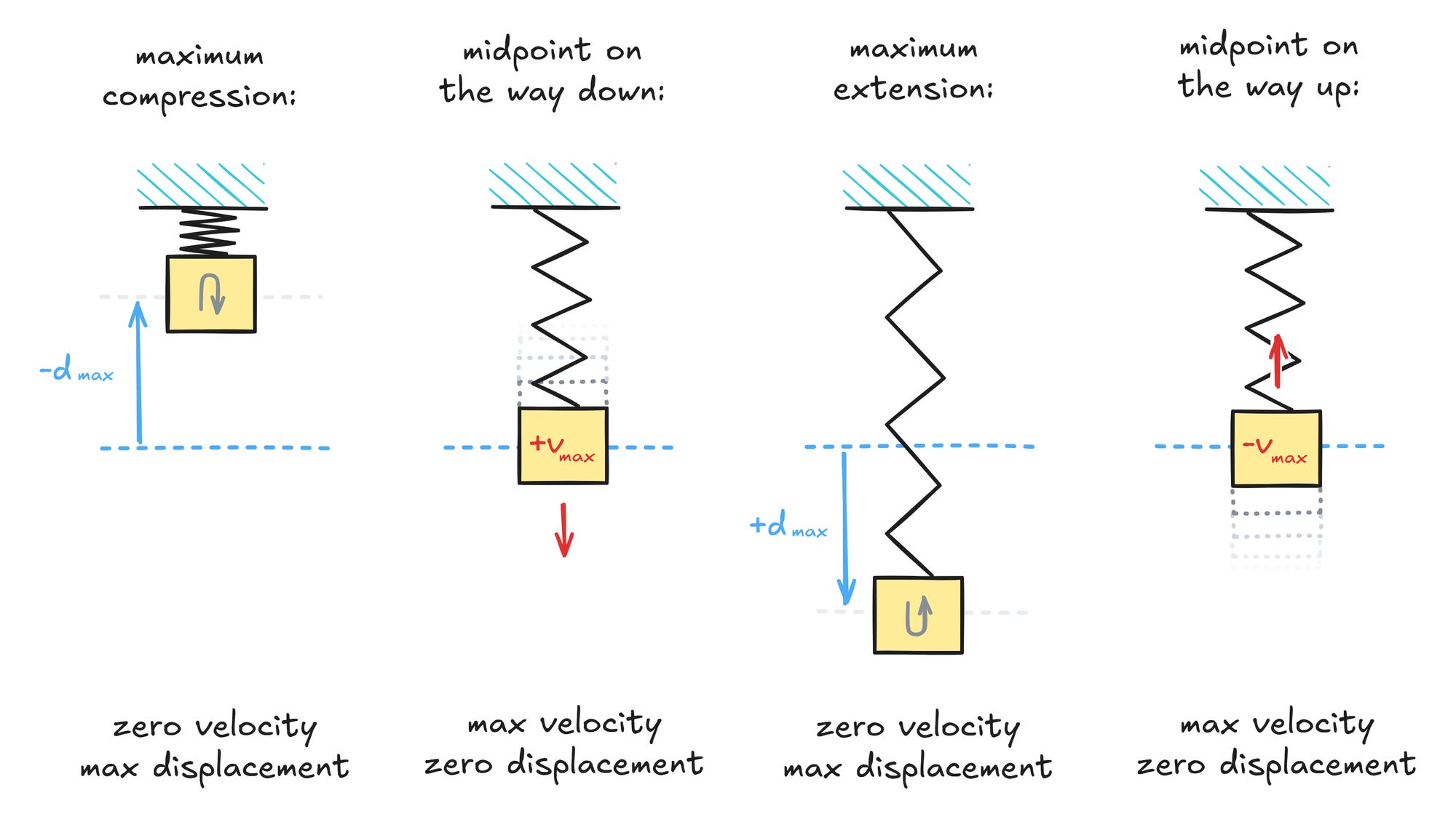
In the diagram, we can spot two interesting boundary conditions. The first one occurs when the spring being maximally compressed or extended; at that point, the velocity of the block is zero and it’s about to reverse direction. The other boundary is reached when spring tension drops to zero at midpoint of the oscillation. At that moment, the block stops being pushed — i.e., accelerated — so this corresponds to its peak velocity.

Note that the description above neglects gravity. For simplicity, we can add “in space!” to the description of the experiment, but informally: gravity doesn’t change the overall dynamics. It’s a constant force acting on the mass, so it just shifts the midpoint condition from “the spring exerts no net force” to “the spring exerts force exactly opposite to gravity”. The block still swings symmetrically from that new midpoint.

And yep: if you plot displacement of the spring (d) or velocity of the block (v) over time, the result will be a sinusoid. But don’t settle for that answer — we still haven’t answered why!

To understand what’s going on, we need to bring up an important yet simple concept in physics: the conservation of energy. In essence, in a closed (i.e., isolated) system, energy can change form — say, from mechanical energy to heat — but the sum of all its forms must remain constant over time.

In this particular experiment, the system is alternating between potential energy stored in a spring and kinetic energy of a moving block. And at all times, the oscillator must adhere to the following rule:

\(E_{total} = E_{spring} + E_{block} = \textrm{const}\)

This equation deals with energy, but that’s not something we can directly observe. We can measure spring deflection and block velocity, but we don’t know how these quantities relate to energy — and even if we peek at Wikipedia, it won’t tell us why.

Energy stored in a spring

The empirical model of a spring is pretty simple: it’s just a linear device that pushes back proportionally to how much you compressed it so far.

More precisely, the momentary “pushback” force you need to overcome (F) to keep compressing the spring is a function of previous displacement (d) and a spring-specific stiffness factor k:

\(F = k \cdot d\)

The value of k depends on the material the spring is made from and its exact shape; for our purposes, we can just assume that it’s some arbitrary constant. If we plot the equation, it’s probably no surprise that we get a straight line:

The behavior of a spring.

Let’s think about what happens if we compress the spring d = 0 to d_max. From the formula above, we know that the force we need to overcome will gradually ramp up from F = 0 to F = k × d_max.

When dealing with a simple linear ramp, we can intuit without calculus that the average force we’ve been pushing with is equal to the midpoint of the graph, i.e.:

\(F_{avg} = {F_{max} \over 2} = {k \cdot d_{max} \over 2}\)

But how does force correspond to energy?

Energy is related to work. If you’re leaning against a stationary lawnmower, you’re exerting force, but no energy is being transferred — and thus, no work is getting done. If you start pushing the lawnmower up a hill by applying a constant force to the handlebars, the situation changes. The amount of work performed — i.e., the amount of energy (E) you expended — is equal to the applied force times the distance traveled (d):

\(E = F \cdot d\)

This also works for pushing a spring! We applied an average force of F_avg to compress the spring by some distance d_max. Combining the formulas, we get:

\(E_{spring} = F_{avg} \cdot d_{max} = {k \cdot {d_{max}}^2 \over 2} \)

Neat: this gives us the potential energy stored in our spring.

Energy of a moving mass

The case of a spring was fairly intuitive; the physics of a moving mass are harder to grok, but we can cheat by bringing up the conservation of energy once more. The trick is that the energy of a moving object must be the same as the energy we transferred to it to accelerate it to that speed.

In other words, if we have a block with a constant mass m, we just need to see how much effort it would take to get it from v = 0 to some given v_max. We can accelerate the object any way we like; two identical objects accelerated in different ways but traveling at the same speed still have the same kinetic energy.

For simplicity, let’s say that we ramped up the speed at a linear rate within t = 1 second. Self-evidently, the resulting acceleration is:

\(a = {v_{max} \over t}\)

Because we ramped up the speed in a straight line from 0 to v_max, it once again follows that the average speed in that one-second time window is:

\(v_{avg} = {v_{max} \over 2}\)

We can now trivially calculate the distance traveled by the mass while being accelerated (d) by multiplying the average speed by the duration of the push:

\(d = v_{avg} \cdot t = {v_{max} \over 2} \cdot t\)

From Newton’s laws of motion, the acceleration of an object is proportional to the applied force and inversely proportional to mass (a = F/m). This should be pretty intuitive, and we can rearrange this to solve for force:

\(F = m \cdot a\)

Substituting the previously-calculated value of a, we get:

\(F = m \cdot {v_{max} \over t}\)

So far, in our toy scenario of trying to accelerate an object any way we like, we calculated the constant force pushing the object (F) and the distance traveled (d). To figure out the work done — and thus, the kinetic energy imparted on the object — we can just plug it into the earlier formula for work (W = F × d):

\(E_{block} = F \cdot d = m \cdot {v_{max} \over \cancel{t}} \cdot {v_{max} \over 2} \cdot \cancel{t} = {m \cdot {v_{max}}^2 \over 2} \)

We end up with an expression for kinetic energy that depends only on velocity and mass.

Right… why are we doing this again?

That’s the neat part. Now, we can rewrite the earlier equation for the conservation of energy as:

\(\begin{align} E_{total} &= E_{spring}+ E_{block} \\ &= {k \over 2} \cdot d^2 + {m \over 2} \cdot v^2 \ ( = \textrm{const}) \end{align}\)

I split out the k/2 and m/2 terms on purpose: they’re just material-specific constants that scale d and v in their respective axes when we plot the observed state of the system. To keep the math tidy, let’s assume that by some stroke of luck, the constants worked out to 1, leaving us with this simplified energy formula:

\(E_{total} = (1 \tfrac{\textrm{N}}{\textrm{m}}) \cdot d^2 + (\textrm{1 kg}) \cdot v^2 = \textrm{const}\)

We can also ignore the units altogether and rewrite the equation in a way that relates the numerical values of displacement and velocity:

\(d^2 + v^2 = \textrm{const}\)

What does this mean in practice? Well, let’s use Cartesian coordinates to plot some arbitrary system state — a randomly-chosen combo of block velocity (v) and spring deflection (d):

Plotting the state of the mass-on-spring oscillator.

We know the values of d and v — we picked them! — but I also added a segment labeled x. It’s the distance from the origin of the coordinate system — (0, 0) — to the point representing system state at (v, d).

The value of x can be calculated from the Pythagorean theorem:

\(x^2 = v^2 + d^2\)

Note the similarity of this expression to the earlier condition for the conservation of energy:

\(d^2 + v^2 = \textrm{const}\)

If the criteria for the conservation of energy in this system is that the sum of these squares (d² + v²) must be constant, then x² must be constant too! And if x² is constant, then it follows that x must be a (different) constant value.

This is an important revelation. It means that all pairs of (v, d) values in a mass-on-a-spring system that obeys the law of conservation of energy must be equidistant to (0, 0). And the set of these equidistant points is… you guessed it, a circle:

A surprise circle, courtesy of thermodynamics.

So, the observable state of our mass-on-a-spring contraption does travel at a constant speed around the circumference of a circle; the circle is just hidden really well.

The rest is triangles

If you already know why this motion would produce a sinusoid, feel free to skip ahead. If not, let’s cover it briefly. The most basic introduction to trigonometric functions is usually done in terms of the relationship between the sides of a right-angle triangle:

The most rudimentary intro to sin(a) and cos(a).

But if the hypotenuse is chosen to have a constant length and if we anchor one end to the center of the coordinate system, then the far end draws a circle as the value of a progresses from 0 to 360°:

The circular parallels.

Meanwhile, the the value of sin(a) corresponds to one of the observable parameters — deflection — in our earlier circle-traveling model of a mass on a spring. The other observable parameter, velocity, is given by the cosine function.

To recap: the reason why the values of v and d are sinusoids if plotted over time is that the observable state of the system is constrained to motion around a circle. But the reason this circle exists is a nuance of the underlying math for the conservation of energy.

In practice, many other natural phenomena have a similar relationship between observable state and energy. For example, a capacitor bears some resemblance to a spring: the more electrons you stored in it, the harder it is to add another — so the stored energy is proportional to the square of charge.

Postscript: is it really constant speed?

Earlier on, I made the following assertion:

“So, the observable state of our mass-on-a-spring contraption does travel at a constant speed around the circumference of a circle; the circle is just hidden really well.”

“But hold on”, some readers said, “how do we know that the speed is constant?”. That’s a good point: if the system is traveling around the circle in some sort of a choppy pattern, the plots of velocity over time or displacement over time wouldn’t be pure sines.

A rigorous explanation is relatively hard to pull off without leaning on prior knowledge of calculus, but one of the readers suggested the following geometric approach that’s pretty easy to grasp:

Calculus without calculus.

The circle on the left is the earlier visualization of system state, with the horizontal axis representing block velocity and vertical axis representing spring displacement.

On the panel on the right, we take a look at the evolution of the system in an infinitesimal time slice (Δt). On a sufficiently microscopic scale — when Δt approaches zero — we can view the local segment of the circle as a straight line. The question we’re trying to answer is whether the incremental distance traveled along the circle (Δs) depends in some way on the momentary value of v or d.

Looking at the small shaded triangle on the right, we can apply the Pythagorean theorem and say the following:

\((\Delta s)^2 = (\Delta v)^2 + (\Delta d)^2\)

So far, so good. Next, let’s ponder what Δd actually is: it’s the increase in displacement over time. And what physical quantity describes the change in position over time? It’s velocity! The incremental displacement of the block — and thus the spring — is proportional to the momentary speed, v, times the duration of the time slice we’re currently looking at:

\(\Delta d = {v \cdot \Delta t}\)

A bit less obviously, Δv works the same way. The increase in speed is proportional to acceleration and time (Δv = a × Δt). Further, as discussed previously, from Newton’s laws of motion, acceleration is directly proportional to applied force (a = F/m); and spring “pushback” force that’s acting on the block is directly proportional to overall displacement (F = k × d). In essence, combining the formulas we talked about earlier in the article, we arrive at:

\(\Delta v = {a \cdot \Delta t} = {F \over m} \cdot \Delta t = {k \cdot d \over m} \cdot \Delta t\)

Both k and m are just scaling constants that squish or stretch the circle; for simplicity, we opted to assume they work out to the same numerical value, the simplified formula boils down to:

\(\Delta v = {d \cdot \Delta t}\)

Now, we can plug these formulas for Δv and Δd into the earlier Pythagorean formula for the small, shaded triangle:

\(\begin{array}{r l} \textrm{Earlier equation:} & (\Delta s)^2 = (\Delta d) ^2 + (\Delta v)^2 \\ \textrm{...substituted:} & (\Delta s)^2 = ({v \cdot \Delta t})^2 + ({d \cdot \Delta t})^2 = (v^2 + d^2) \cdot (\Delta t)^2 \\ \textrm{...simplified:} & \Delta s = \sqrt{v^2 + d^2} \cdot \Delta t \end{array}\)

Recall that the main thrust of our earlier proof for “circularity” was that v² + d² = const. So, when Δt is vanishingly small, the rate at which the system advances along the circle is proportional to a constant multiplied by Δt.

QED.

👉 For a bit more basic physics nerdery, check out the articles on the physics of conduction, the behavior of transistors, and on core concepts in electronic circuits. For the best damn intro to the discrete Fourier transform, click here.

---

I write well-researched, original articles about geek culture, electronic circuit design, and more. If you like the content, please subscribe. It’s increasingly difficult to stay in touch with readers via social media; my typical post on X is shown to less than 5% of my followers and gets a ~0.2% clickthrough rate.