Approximation game

The number 22/7 and the pigeon flocks of Peter Gustav Lejeune Dirichlet

In some of the earlier articles on this blog, we talked about the nature of real numbers and the meanings of infinity. The theory outlined in these posts is interesting but also hopelessly abstract. It’s as if we’re inventing make-believe worlds that have no discernible connection to reality.

In today’s post, we’ll examine a cool counterexample: an outcome of an numerical experiment that can be backed up with fairly simple proofs, but that makes sense only if you take a step back to consider the construction of real numbers and rationals.

We start by picking a real number r. Your job is to approximate it as closely as possible using a rational fraction a / b with a reasonably small denominator. The approximation can’t be the same as r. Is this task easier if r itself is rational or irrational?

Make a guess and let’s dive in. For simplicity, we’ll stick to a positive r and positive fraction denominators throughout the article.

Defining “good”

For a chosen denominator b, it’s pretty easy to find the value of a that gets us the closest to the target r. We must consider two cases: the largest “low-side” fraction that’s still less than r; and the smallest “high-side” fraction greater than r. If there’s a rational fraction that matches r exactly, that solution is prohibited by the rules of the game; we need to pick one of the nearby values instead.

If you wanted to find an exact match, you could try a_ideal = r · b; this makes the a / b fraction equal to r · b / b = r. That said, r · b might not be an integer (or even a rational number), so even without the added “no exact matches” rule, the approach is usually a bust.

If we round the value up (⌈r · b⌉), we get a number that is equal or greater than a_ideal; if it’s greater, the difference between the two values will be less than 1. In other words, we can write the following inequality:

\(a_{ideal} \leq\lceil r · b\rceil < a_{ideal} + 1\)

This is saying that the rounded-up number may be equal to the ideal solution needed to match r exactly, or it might overshoot the target, but always by less than the minimum possible increment of the numerator in the a / b fraction.

The result is almost what we need, but once more, the rules prohibit approximations that are exactly equal to r. The workaround is to subtract 1 from all sides of the inequality:

\(a_{ideal} - 1 \leq \lceil r · b \rceil -1 < a_{ideal}\)

The effectively tells us that the middle term — ⌈r · b⌉ - 1 — is always less than the value needed to match r, but the difference is never greater than a single tick of the numerator. We’re as close as we can be; the value of a for the optimal low-side approximation (a / b < r) is:

\(a_{low} = \lceil r \cdot b \rceil - 1 \)

We can follow the same thought process to find the high-side estimate (a / b > r); this time, we round the product down and then add 1:

\(a_{high} = \lfloor r \cdot b \rfloor + 1 \)

Finally, the error (ε) associated with any a / b can be easily calculated as:

\(\varepsilon = \biggl|r - \frac{a}{b}\biggr|\)

We have previously established that if we pick a_low or a_high, the error can’t exceed one tick of the numerator, which works out to ± 1/b. As a practical example, if we’re trying to approximate r = 2 using b = 5, the best inexact solutions are 9/5 = 1.8 on the low side and 11/5 = 2.2 on the high side; they both have an error of 1/b = 0.2.

Next, we’ll try to examine if the error can be less. If we find any approximations that are better than the worst-case scenario — i.e., that satisfy ε < 1/b — we’re gonna call them 1-good.

As an inspection aid, we can also define a normalized score s calculated by multiplying ε by b:

\(s = \varepsilon \cdot b\)

The equation keeps the maximum error at 1 regardless of the denominator we’ve chosen. By that metric, a 1-good approximation is associated with s < 1.

The rational test case

Now that we have the mechanics spelled out, let’s take r = 1/4 and analyze the optimal solutions for some initial values of b:

\(\begin{array}{|r|c|c|c|l|} \hline \mathbf{b} & \textbf{Best a/b} & \textbf{Error (ε)} & \textbf{Score }\mathbf{(s)} & \textbf{1-good?} \\ \hline 1 & 0/1 & 1/4 & 1/4 & yes\\ \hline 2 & 0/2 & 1/4 & 1/2 & yes\\ \hline 3 & 1/3 & 1/12 & 1/4 & yes \\ \hline 4 & 0/4 & 1/4 & 1 & no \\ \hline 5 & 1/5 & 1/20 & 1/4 & yes \\ \hline 6 & 2/6 & 1/12 & 1/2 & yes\\ \hline 7 & 2/7 & 1/28 & 1/4 & yes\\ \hline 8 & 1/8 & 1/8 & 1 & no\\ \hline 9 & 2/9 & 1/36 & 1/4 & yes\\ \hline 10 & 2/10 & 1/20 & 1/2 & yes\\ \hline \end{array}\)

We find that many approximations are 1-good (ε < 1/b, s < 1) and outperform their peers; for example, 1/5 = 0.2 is better than 2/6 ≈ 0.333. Nevertheless, the results are underwhelming: the values diverge from the 1/b baseline by small factors that are stuck on repeat. If we plot a larger sample, we get:

Approximation scores for r = 1/4.

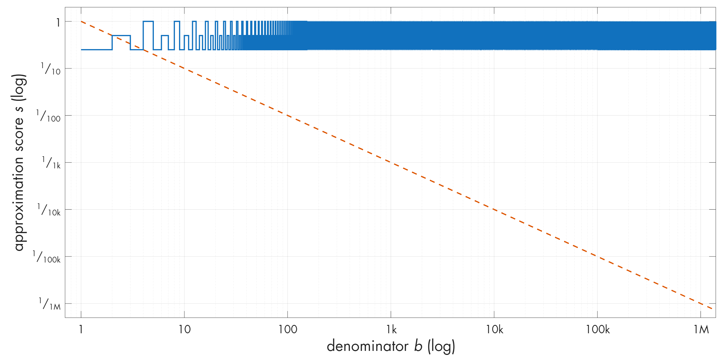
In this log-scale plot, I also included a diagonal line that represents error values decreasing with the square of the denominator (1/b²). Approximations for which the error dips below this line would be markedly better than the ones that merely dip below 1/b. We can label these 1/b² solutions as 2-good.

In the plot, we see two trivial approximations below the 2-good line, but for a rational r, we can prove that the effect can’t last. We start by rewriting r as a fraction of two integers: r = p / q. The 2-goodness criteria is ε < 1/b². We’ve previously defined ε = | r - a/b | and per the rules of the game, valid solutions must have ε greater than zero. Putting it all together, we can write this inequality that spells out the requirements for 2-good approximations of rationals:

\(0 < \biggl| \frac{p}{q} - \frac{a}{b}\biggr| < \frac{1}{b^2}\)

To tidy up, we can bring the middle part to a common denominator:

\(0 < \biggl| \frac{b\cdot p - a \cdot q}{b \cdot q}\biggr| < \frac{1}{b^2}\)

The denominator is positive, so there’s no harm in taking it out of the absolute-value section and multiplying all sides of the inequality by it:

\(0 < \bigl|b \cdot p - a \cdot q \bigr|< \frac{q}{b}\)

All the variables here are integers. If b ≥ q, the fraction on the right is necessarily ≤ 1. That creates an issue because it implies the following:

\(0 < \bigl|b \cdot p - a \cdot q \bigr|< 1\)

Again, the middle section comprises of integers, so it can’t possibly net fractions. In effect, the equality says: 0 < integer < 1; there’s no integer that satisfies this criterion, so the assumption of b ≥ q leads to a contradiction. If any inexact 2-good approximations of rational numbers exist, they can only exist for b < q.

That’s where we look next. If the target real r = p / q is given at the start, then q doesn’t change and the b < q condition restricts the solutions to integer a / b fractions with smaller denominators. There’s only a finite number of these.

To address one natural objection, we don’t get more latitude for b by rewriting r to use proportionately greater q and p — for example, restating r = 1/2 as r = 4/8. If we do that, we go from the original inequality:

\(0 < \bigl|b \cdot p - a \cdot q \bigr|< \frac{q}{b}\)

…to:

\(0 < \bigl|b \cdot {4} p - a \cdot {4} q \bigr|< \frac{{4} q}{b}\)

If you divide all sides by 4, you end up where you started, so the trick accomplished nothing at all. In effect, if any 2-good approximations of a rational number r exist, there can’t be more of them than allowed by the b < q criteria for the lowest-terms representation of r = p / q. And these solutions, if any, will be clustered on the left side of the plot.

This is about as much as we can squeeze out of that stone. The bottom line is that rational numbers are difficult to approximate using other rationals; in fact, the simpler the number, the fewer good approximations we get.

Approximating irrationals

If rationals tend to be relatively resistant to approximations, it might be tempting to assume that the situation with irrational numbers is going to be worse. But, to cut to the chase, here’s the plot of approximations for r = π:

Approximation scores for r = π.

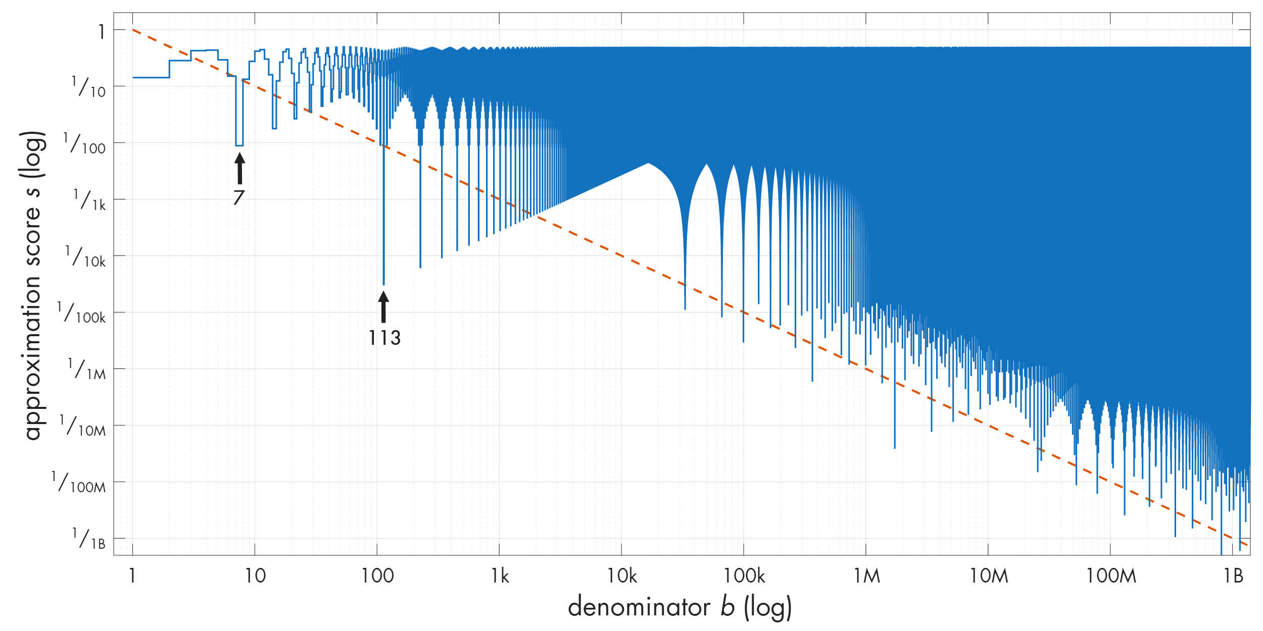
Note that the plot keeps dipping below the 2-good line over and over again. And there are some really nice approximations in there! The first arrow points to 22 / 7 ≈ 3.143 (s ≈ 0.009). The second arrow points to an even better one: 355 / 113 ≈ 3.141593 (s ≈ 0.00003). What’s up with that?

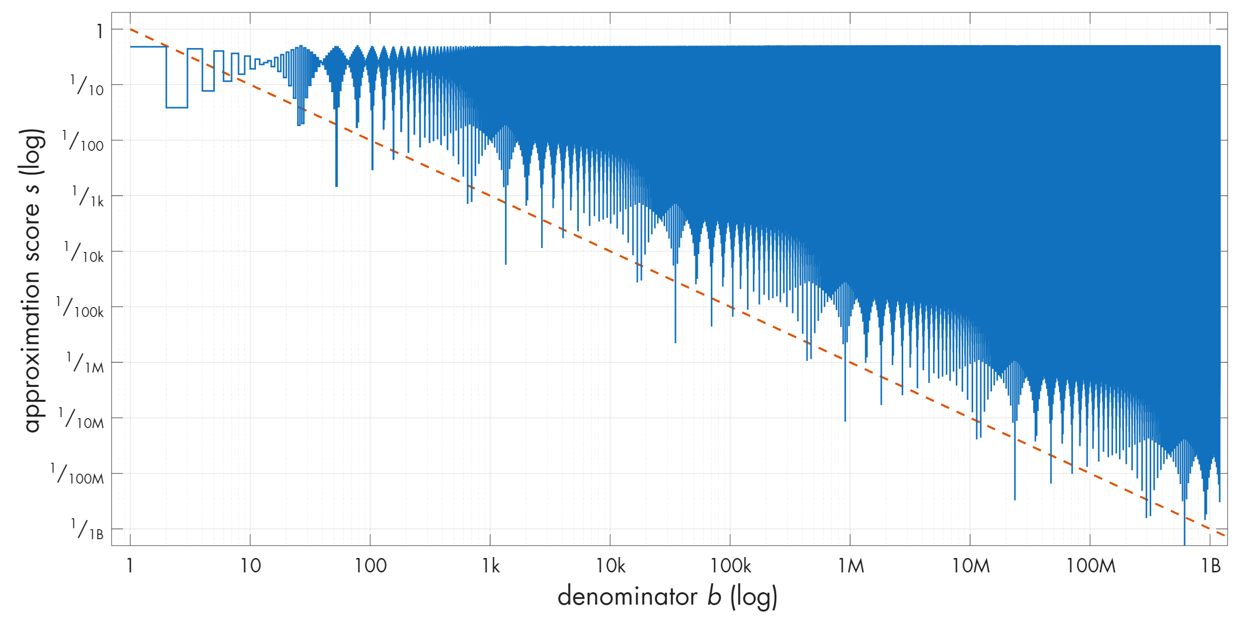
Before we investigate, let’s confirm that π is not special. Surely enough, these patterns crop up for other irrationals too. And it’s not just famous transcendental constants; here’s √42:

Approximating r = √42.

To understand what’s going on, we need to build a lengthier proof, although we’ll still stay within the realm of middle-school math.

First, we make a simple observation: given some number r, we can always split that number into an integer part v and a fractional part x that satisfies 0 ≤ x < 1. In other words, we’re rewriting r as v + x such that x falls in the interval [0, 1).

We can also deconstruct any multiple of r the same way. In particular, we can calculate k · r for every integer k between 0 and some arbitrary upper bound K > 0; for each of the resulting values, we can then split the result to obtain a sequence of integer parts (v₀ to v_K) and fractional parts (x₀ to x_K). A simple illustration of this idea for π is:

\(\begin{alignat}{1} 0 \cdot \pi \quad &\rightarrow \quad v_0 = 0, &&x_0 = 0 \\ 1 \cdot \pi \quad &\rightarrow \quad v_1 = 3, &&x_1 = 0.1415\ldots \\ 2 \cdot \pi \quad &\rightarrow \quad v_2 = 6, &&x_2 = 0.2831\ldots \\ 3 \cdot \pi \quad &\rightarrow \quad v_3 = 9, \quad &&x_3 = 0.4247\ldots \\ &\ldots \end{alignat}\)

These integer and fractional sequences both have K + 1 elements because we started counting at zero — and again, each fractional part falls somewhere in the interval [0, 1).

Next, we divide the [0, 1) interval into K sub-intervals (“buckets”) of equal size:

\(\underbrace{\biggl[0, \; \frac{1}{K}\biggr)}_\textrm{bucket 1}, \; \underbrace{\biggl[\frac{1}{K}, \; \frac{2}{K}\biggr)}_\textrm{bucket 2}, \; \ldots \;, \; \underbrace{\biggl[\frac{K-1}{K}, \; 1\biggr)}_\textrm{bucket K}\)

We have K buckets and K + 1 fractional x values that are distributed across these buckets; no matter how we slice and dice it, at least two x values will necessarily end up in the same bucket. This is the pigeonhole principle.

Again, the reasoning implies that there’s at least one pair of indices, g < h, such that x_g and x_h both ended up in the same bucket. We don’t know anything about the underlying numbers, except that by the virtue of where they landed, they must be less than the width of the bucket (1 / K) apart:

\(\bigl|x_h - x_g\bigr| < \frac{1}{K}\)

The inevitability of a pair of elements with spacing of less than 1 / K is the crux of the proof. The rest is just a bit of manipulation to relate these elements to a rational approximation of the starting number r.

We show this in a couple of steps. First, as a consequence of how we constructed these fractional parts, we can rewrite any x_k as the difference between the k-th multiple of r and the associated integer part v_k. After making these substitutions for indices h and g, we get:

\(\bigl| \underbrace{h \cdot r - v_h}_{x_h} - (\underbrace{g \cdot r - v_g}_{x_g}) \bigr| < \frac{1}{K}\)

Next, we group the r-coupled and r-free terms, obtaining what appears to be two independent integers: (v_h - v_g) and (h - g). We label these a and b:

\(\bigl| r \cdot \underbrace{(h - g)}_b - \underbrace{(v_h - v_g)}_a \bigr| < \frac{1}{K}\)

We don’t need to dwell on the possible values of a; it’s enough that the number can exist. We’re also not concerned about the exact value of b, although we ought to note that it’s always positive (because we specified g < h) and that it’s necessarily less than or equal to K (because it represents the difference of indices in a list with K + 1 elements).

We’ll lean on these properties soon, but for now, let’s bake a and b into the earlier inequality to obtain:

\(\bigl| r \cdot b - a \bigr| < \frac{1}{K} \quad \textrm{(⚑)}\)

Remember the flag for later and divide both sides by b to obtain:

\({\bigl| r - \frac{a}{b} \bigr|}< \frac{1}{K\cdot b}\)

Huh — the left-hand portion of the expression is the same as the formula for the error ε of approximating r using a rational fraction a / b. In other words, the inequality seems to be saying that, as a consequence of the pigeonhole principle, we can pick any r and any K > 0, and there’s always some integer a / b that approximates r with an error of less than 1 / (K · b).

We haven’t picked any specific K, but we know that b is always less or equal than K; again, this is because we defined b as a substitution for h - g, the delta between two indices in a sequence of K + 1 elements. Therefore, the expression in the denominator — K · b — involves multiplying b by a value that’s equal or greater than b. In effect, we have proof that for any real r, some a / b satisfies ε < 1/b².

This proof is known as Dirichlet’s approximation theorem. At first blush, it only guarantees a single 2-good approximation for every real. Worse yet, the solution guaranteed by the proof might not comply with the rules of our game, because nothing stops it from producing exact approximations (ε = 0). So, what did we achieve?

Well, that’s where we come back to an intermediate equation marked with ⚑:

\(\bigl| r \cdot b - a \bigr| < \frac{1}{K} \\\)

In the earlier course of the proof, we divided the left-hand side of this inequality by b to arrive at the formula identical to ε. Equivalently, we can say that the current form is equal to ε · b. We already have a name for this parameter: this is the normalized approximation error s, as introduced early in the article.

We can also assert that for any irrational r, this normalized error must be greater than zero. To prove this property, it’s sufficient to show that we’d end up with a contradiction if multiplying r by a positive integer (b) produced some sort of a rational number — an ad hoc fraction h / j, where h and j are also integers. If r · b = h / j, we can represent r itself as a fraction, making it rational:

\(r \cdot b = \frac{h}{j} \quad \implies \quad r = \frac{h}{j \cdot b}\)

In other words, if r is irrational, the same must hold for r · b. Since r · b is an irrational number and not an integer, subtracting an integer from it will always leave a fractional part. Therefore, s = | r · b - a | must be > 0.

To take the next step — and we’re close to the finish line! — note that Dirichlet’s proof doesn’t put any constraint on the upper value on the number of buckets (K). If we choose some specific K₁, the earlier proof establishes the existence of a single 2-good pair, which we can label a₁ and b₁. If we choose another value K₂, the proof establishes the existence of a potentially different pair we’ll call a₂ and b₂. That said, who knows if the pairs actually differ? Maybe there’s just a single solution that repeats for every K?…

Let’s assume that’s the case; if the resulting approximations are identical, the same goes for the normalized approximation error: s = s₁ = s₂. In this scenario, we’re entertaining the possibility that this single value satisfies the flagged inequality in both proofs: s < 1 / K₁ and s < 1 / K₂.

At the same time, we have noted that in the irrational case, s must be positive. Real numbers can be arbitrarily small, but they can’t be infinitely small, so for any positive s that obeys the first inequality, we can make the 1 / K₂ fraction in the second proof smaller than s simply by choosing a sufficiently large K₂. This leads to a contradiction. We must conclude that, for some K₂ > K₁, we necessarily get a new, better approximation (s₂ < s₁).

Further, if we keep incrementing K, this new a₂ / b₂ approximation will eventually succumb to the same fate. We can evidently get as many 2-good pairs as we want. The proof doesn’t guarantee that it’s going to happen on any specific cadence, but it says that the outcome is inevitable.

As a postscript, we ought to ask if the same reasoning applies to rationals; if it does, that would contradict our earlier argument that rational numbers can only have a handful of 2-good solutions. To show that there is no contradiction, note that in the rational case, s can conceivably reach zero (i.e., there is some a / b value that is an exact approximation). The rules of our game reject these approximations, but as discussed earlier, the constraint is not baked into Dirichlet’s proof.

Next, rewrite r as p / q in the left-hand portion of the earlier inequality:

\(\biggl| r \cdot b - a \biggr| = \biggl| \frac{p}{q} \cdot b - a \biggr| = \biggl| \frac{b \cdot p - a \cdot q}{q} \biggr| \)

The numerator of the fraction on the right is an integer (because so are a, b, p, and q). The denominator is also an integer that stays constant for a given r. It follows that when approximating rationals, there is a fixed, minimum decrement for s: 1/q. We might start from a non-zero s₁, but if we keep ramping up K, the system must reach the degenerate s_n = 0 case after producing a finite number of inexact approximations. From that point on, s < 1 / K is satisfied for any K and the proof no longer necessitates the generation of additional 2-good pairs.

As before, we can’t cheat by increasing p in tandem with q (e.g., r = 1/2 to r = 4/8). This trick increments the nominator and the denominator by the same factor, still producing the same effective step; the solution is predicated on the lowest-terms representation of r = p / q.

In the end, you get an infinite supply of surprisingly accurate solutions for irrational numbers, but a limited (often very limited) number of decent results for rationals.

But… why?

Right. The proofs are interesting but don’t offer an intuitive explanation of why these patterns emerge. This is where we go back to my opening remark: it’s easier to grasp the outcome if you look at how rational numbers and reals are “made”.

From the construction of rationals, we know that the spacing between them is arbitrarily close, but at any “magnification level” — for any chosen denominator b — the values divide the continuum into uniform intervals. Uniform spacing also implies maximal spacing: even though there is no upper or lower bound to the values of a / b, they are as far apart as they can be. Any new value inserted onto the number line will necessarily sit “closer” to an existing rational.

The gaps between rational numbers is where we find irrationals. This comes with a lot of weird baggage explored in the previous article, but it also means that for any given irrational r, we have an inexhaustible supply of unexpectedly accurate rational approximations in the vicinity.

Although the puzzle we started with might seem silly, the study of these structures — known as Diophantine approximations — is taken seriously and gets complicated fast. For example, it’s possible to construct so-called Liouville numbers that have an infinite irrationality exponent (endless n-good approximations for any n), but it’s a lot harder to prove that any commonly-encountered number has an irrationality exponent greater than two. In the same vein, algebraic irrationals (e.g., √2) all have an irrationality measure of two, but the proof of this is fiendishly difficult and netted its discoverer the Fields Medal back in 1958.

---

You might also enjoy my other articles about math, including:

How many dimensions is this?

Folks, we have the best π

You gotta think outside the hypercube

I write well-researched, original articles about geek culture, electronic circuit design, algorithms, and more. If you like the content, please subscribe.