Unreal numbers

Reals are really weird.

A while ago, I posted an article about the 19th and early 20th century quest to derive mathematics from the principles of formal logic. We kicked off with Peano arithmetic, which built natural numbers from two ad-hoc constructs: an element representing zero and an abstract “successor” function S(…).

Later, we leaned on set theory to encode the underlying structure of these symbols. This netted us a hierarchy of set-theoretic natural numbers known as ordinals. It also led to an interesting insight: if we allowed the existence of infinite sets, then the set of all natural numbers (ℕ) itself had the structure of an ordinal. In the article, we labeled this infinite number ω and demonstrated that it could be manipulated using the same arithmetic rules as finite numbers, but that it sometimes behaved in wacky ways. For example, we established that ω + 1 ≠ 1 + ω.

We also touched on various methods of reasoning about the magnitude of ordinals and showed that these approaches diverge from each other in the realm of infinities. In particular, we talked about Georg Cantor’s notion of cardinality, which put many distinct infinite ordinals in the same size class, but indicated that there’s a fundamental difference in scale between the set of natural numbers and the set of reals (ℝ).

If you haven’t read the article but are intrigued, I strongly encourage you to give it a go (link). I think it’s an excellent and accessible introduction. If you’re up to speed, there might be one thing that’s bugging you: we carefully defined natural numbers from first principles, but then pulled reals out of a hat. This is a gap worth addressing, because as it turns out, real numbers are profoundly weird.

Natural numbers (ℕ)

As a reminder, in the earlier article, we constructed a succession of natural numbers by conjuring an object representing zero and then successively applying function S(…) to it:

\(\begin{align} 1 &:= S(0) \\ 2 &:= S(1) = S(S(0)) \\ 3 &:= S(2) = S(S(S(0))) \\ 4 &:= S(3) = S(S(S(S(0)))) \\ &... \end{align} \)

The “:=” operator means “is defined as”. Elsewhere, you might see this written as ≝, ≜, or a regular =.

In Peano arithmetic, the label “0” and the successor function S(…) have no deeper meaning: they are just “things” with a couple of common-sense properties spelled out. All the notation indicates is that every subsequent label has some fixed relationship to the one that came before. In the set-theoretic approach we switched to later, we defined these concepts with more precision, but this detail doesn’t matter now.

The important point is that in both models, the successor relationship allowed us to define the behavior of the “+” operator using a pair of simple substitution rules:

\(\begin{alignat}{1} a &+ 0 \;&&:=\; a&&\qquad (\textrm{rule 1}) \\ a &+ S(b) \;&&:=\; S(a+b) &&\qquad ( \textrm{rule 2}) \end{alignat}\)

Although the rules may seem cryptic, they effectively just codify that adding zero is a no-op and that a + (b + 1) is the same as as (a + b) + 1.

This ruleset lets anyone solve problems such as 2 + 2 without any assumptions about the fundamental meaning of “2” or “+”. To illustrate, from the definition of Peano numbers, we note that “2” is the same as S(1), so 2 + 2 can be restated as 2 + S(1). Switching to that form allows us to apply rule #2, in turn rewriting 2 + S(1) as S(2 + 1):

\(2 + 2 = 2 + S(1) = S(2 + 1)\)

After that, we can apply the same steps again to expand the nested 2 + 1 sum:

\(S(2+1) = S(2 + S(0)) = S(S(2 + 0))\)

We now have a doubly-nested sum involving zero, so we can apply rule #1, getting rid of the sum (2 + 0 = 2) and “unwinding” the successor functions to arrive at the result:

\(2 + 2 = S(S(2+0)) = S(S(2)) = S(3) = 4\)

Again, if you’re interested in a more detailed walkthrough, including C code that explains the process in programmer-friendly terms, check out the article linked earlier on.

What we haven’t covered in that article is that we can use a similar approach to recursively define multiplication for natural numbers:

\(\begin{alignat}{1} a &\cdot 0 \;&&:=\; 0 &&\qquad (\textrm{rule 1}) \\ a & \cdot S(b) \;&&:=\; a \cdot b + a &&\qquad ( \textrm{rule 2}) \end{alignat}\)

In effect, without having to explicitly define subtraction, we’re saying that a · b can be rewritten as a · (b-1) + a, and that this expansion should be continued until we get to a · 0. At that point, the multiplication part works out to zero, so we just unwind the stack and gather all the “+ a” terms. This will come in handy in a while.

Integers (ℤ)

A major hurdle on our path toward a complete system of arithmetic is that natural numbers can’t represent negative values. This means that if we attempt to define subtraction, many results will not have an in-system representation, throwing a wrench in the works.

To extend ℕ to negative numbers, we could futz around with a way to encode the minus sign and then special-case it in the arithmetic rulesets. That said, a better-behaved approach is to define integers as a separate hierarchy of numbers, each integer i consisting of an ordered pair of naturals: i = (a, b). The first element of the pair represents the positive component while the second represents the negative part. That is, integer +5 can be encoded as (5, 0) while integer -5 becomes (0, 5).

You might be wondering if we just pulled the concept of an “ordered pair” out of thin air. Yes and no: it’s new here, but in set theory, these pairs are mapped to normal sets, except we design the mapping so that (a, b) differs from (b, a). This can be done in a number of ways, but a common approach devised by Kazimierz Kuratowski is:

\((a, b) := \{ \{a\}, \{a, b\} \} \)

In essence, the pair is represented by a two-element set, but the second element also embeds a copy of the first, so the result is different depending on the order of the elements in the pair. This encoding has a couple of nice properties, but they’re not important to what we’re about to do.

To define the addition of pair-based integers, we can simply add the “positive” and “negative” halves separately. Since the underlying elements are natural numbers, we already know how to add them, and we can write:

\( \underbrace{(a, b)}_{\textrm{integer 1}} + \underbrace{(c, d)}_{\textrm{integer 2}} \; := \; \underbrace{(\;\overbrace{\vphantom{|}a + c}^{\substack{\textrm{natural} \\ \textrm{addition}}}, \; \overbrace{\vphantom{|}b + d}^{\substack{\textrm{natural} \\ \textrm{addition}}}\;)}_{\textrm{integer result}}\)

In the same vein, because each integer effectively expresses the difference between two underlying numbers, the result of multiplying two integers (a, b) and (c, d) will follow the school-taught pattern of (a - b) · (c - d) = ac - ad - bc + bd. We split out the positive and negative parts of the solution and write:

\(\underbrace{(a, b)}_{\textrm{integer 1}} \cdot \underbrace{(c, d)}_{\textrm{integer 2}} \; := \; \underbrace{(ac+ bd, ad + bc)}_{\textrm{integer result}}\)

These rules work, sort of. For example, adding integer +5 and -5 nets us:

\((5, 0) + (0, 5) = (5 + 0, 0 + 5) = (5, 5)\)

The result (5, 5) seems to be saying “zero”, but is not what we’d choose as the canonical representation of that value; we would have preferred (0, 0). More generally, we’d say that any two pairs (a, b) and (c, d) represent the same integer if a - b = c - d. Yet, our system doesn’t take this property into account.

Because we still haven’t defined subtraction, we must first shuffle the terms around to express the “sameness” criterion in terms of addition:

\(a + d = c + b\)

With this pair equivalence relationship defined, we assign integer labels such as “+5” not to a specific pair, but to an entire equivalence class: a collection of ordered pairs that satisfy the same criteria. In this model, our new hierarchy of numbers looks the following way:

\(\begin{array}{| r | l | l |} \hline \textbf{Integer label} & \textbf{Equivalence class} & \textbf{Class members} \\ \hline {-2} & [(n, n+2)] & (0, 2), (1, 3), (2, 4) \ldots \\ \hline {-1} & [(n, n+1)] & (0, 1), (1, 2), (2, 3) \ldots \\ \hline {0} & [(n, n)] & (0, 0), (1,1), (2,2) \ldots \\ \hline {+1} & [(n+1, n)] & (1,0), (2,1), (3,2) \ldots \\ \hline {+2} & [(n+2, n)] & (2, 0), (3,1), (4,2) \ldots \\ \hline \end{array} \)

We’re mostly done with integers, but before we wrap up, let’s ponder if the set of integers is “larger” than the set of natural numbers. By some metrics, you could argue it is. That said, using the method outlined in the earlier article, every integer can be mapped to a natural number without the risk of running out of naturals:

A simple mapping between ℤ and ℕ.

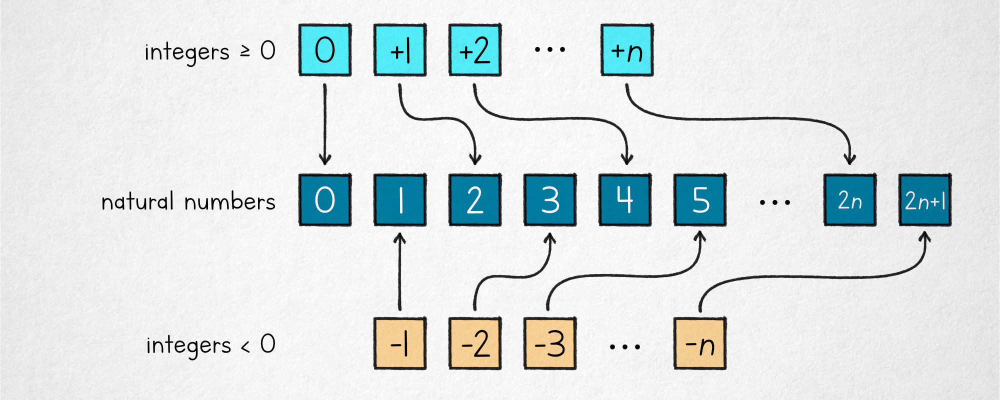
This is because every element in these sets is finite but there is no upper bound; for any finite +n, the number 2n is also finite and has a place in ℕ. We can find a one-to-one mapping between the sets, so we say that the sets have the same cardinality.

Rationals (ℚ)

Rational numbers are values that can be expressed as a ratio of two integers: a / b. In the previous section, we defined integers using an ordered pair that effectively encoded subtraction: a - b. So, here’s the cool part: nothing stops us from taking two integers and fashioning them into a new type of a pair that encodes division. Each of these integer pairs forms a new hierarchy of rational numbers: q = (a, b).

In this model, we consider rationals (a, b) and (c, d) to be equivalent if the underlying integers satisfy the criterion a / b = c / d. We don’t have division defined yet, but we know how to multiply integers, so we can restate the equivalence rule as:

\(a \cdot d = c \cdot b\)

This nets us the following taxonomy:

\(\begin{array}{| r | l | l |} \hline \textbf{Rational label} & \textbf{Equivalence class} & \textbf{Class members} \\ \hline 2/3 & [(2n, 3n)] & (+2,+3), (-2,-3), (+4,+6) \ldots \\ \hline 1/1 & [(n, n)] & (+1,+1), (-1,-1), (+2,+2) \ldots \\ \hline 3/2 & [(3n, 2n)] & (+3,+2), (-3, -2), (+6,+4) \ldots \\ \hline \end{array} \)

The multiplication rule for two pairs representing rational numbers is just a trivial restatement of a/b · c/d = ac/(bd):

\(\underbrace{(a, b)}_{\textrm{rational 1}} \cdot \underbrace{(c, d)}_{\textrm{rational 2}} \; := \;\underbrace{(a \cdot c, b \cdot d)}_{\textrm{rational result}}\)

The addition of rationals is equally straightforward and follows the normal a/b + c/d = (ad + cb) / (bd) pattern:

\(\underbrace{(a, b)}_{\textrm{rational 1}} + \underbrace{(c, d)}_{\textrm{rational 2}} \; := \; \underbrace{(ad + cb, bd)}_{\textrm{rational result}}\)

What’s the “size” of ℚ? Well, again, depends on how we look at it, but we can show that the cardinality of is not greater than ℕ. One visual approach is to construct a two-dimensional array of fractions in the form of x/y:

Laying out and traversing ℚ.

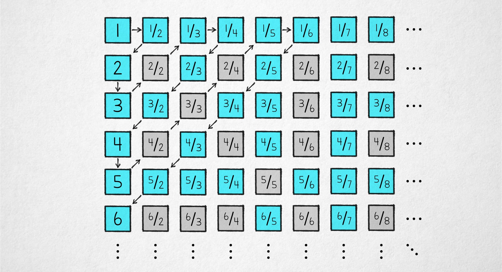
It should be evident that because x and y coordinates separately go through every possible natural number, the array contains all positive rational fractions. Some of the tiles are redundant (e.g., 2 is the same as 4/2), but this is not important for the proof.

With the rationals laid out, we can traverse this grid in a way that lets us assign every tile to an integer without leaving any gaps and without ever running out of members of ℕ. The start of one such traversal pattern is indicated by arrows in the figure. We begin in the top left corner, move one tile to the right, take a a sharp turn to and start moving diagonally until we hit the vertical edge, move one tile down, and then follow a diagonal pattern back. Rinse, repeat. By analogy to what we’ve done for integers, the result doesn’t change if we toss negative rationals into the mix.

Computable numbers

Not every number can be expressed as an integer fraction. The two examples of irrational numbers that every reader should be familiar with are √2, which can be expressed in polynomial terms, and π, which cannot.

Although these numbers can’t be represented as simple fractions, they can be explained in terms of an algorithm you need to follow to approximate them to an arbitrary degree. For example, the sum of the following terms starting at n = 0 will slowly but surely converge to π as the count of summed elements grows:

\({8 \over (4n + 1)(4n + 3)}\)

Within the bounds of the precision of floating-point numbers, you can observe the behavior by running the following C code (demo link):

#include <stdio.h>
#include <stdint.h>

int main() {
  double sum = 0;
  for (uint64_t n = 0, pos = 0; n <= 65536; n++) {
    sum += 8.0 / ((4*n + 1) * (4*n + 3));
    if (n >> pos) { printf("[%5ld] %.05f\n", n, sum); pos++; }
  }
}

At first blush, it would appear that any well-specified irrational number of our choice can be expressed as an approximation algorithm. This leads to a concept that should appeal to any geek: computable numbers. It’s the set of all numbers that can be approximated to an arbitrary precision in finite time by a theoretical model of a computer known as a Turing machine. In effect, the number is the algorithm.

Interestingly, the cardinality of the set of computable numbers is still the same as the cardinality of ℕ. An intuitive explanation is that there are only as many computable numbers as there are Turing machines that could generate them. The ruleset of every Turing machine can be encoded as a finite natural number — you could just write it down and then convert the spec to ASCII values — so we’re still in the realm of countable infinities.

Reals (ℝ)

Of course, we don’t teach about computable numbers in school. Instead, the most common “upgrade” from ℚ are reals: an idealized continuum on which, to put it in a hand-wavy way, every number exists whether we know how to algorithmically approximate it or not.

Now, my phrasing here is severely deficient. It’s not a free-for-all: 🥔 (a potato) is not a real number, and to avoid a variety of complications, neither is √-1. The set ℝ extends ℚ, but it does so only in the immediate vicinity of rationals. Pick any real and I can find a rational fraction that’s arbitrarily close.

To describe the underlying structure of real numbers, we can turn to Dedekind cuts. Informally, the idea is that we can unambiguously identify each real number by associating it with the set of all rationals that come before it. To describe real number x, we could take the set of rational numbers and partition it into an ordered pair of sets (A, B), such that set A contains every rational q < x and set B contains every q ≥ x.

This description may seem circular: to build the representation of a real number, we need to know where to make the cut, which seem to require some prior knowledge about how x relates to ℚ. That said, the point isn’t that the method lets you find the exact spot for π; it’s that the universe of real numbers is built by taking every possible Dedekind cut of ℚ. The numbers are the cuts, and π is somewhere out there, even if we can’t easily pinpoint its location.

To be fair, for some irrational numbers, we can describe the partition in pretty intuitive terms. For example, to describe the cut associated with ∛5, we can say that set A consists of every rational q such that q³ < 5 and set B contains every q such that q³ ≥ 5. It’s a pretty usable specification, but again: the existence of a real number doesn’t depend on us being able to say where it lies.

Once we have numbers expressed in terms of Dedekind cuts, we can define arithmetic operations on reals, too. For example, to add real (A, B) to (C, D), we construct a new number (E, F) such that for every possible rational a selected from A and every rational c selected from C, the sum a + c is placed in E. In the same vein, for every b in B and d in D, the sum b + d goes into F.

I’ll spare you the abstract set notation, but as a practical example, if (A, B) represents 2 and (C, D) represents 3, we know that every a selected from A will be less than 2 and every c chosen from C will be less than 3. Therefore, every a + c value placed in E will be always less than 5. Similarly, every b + d that goes into F will be greater or equal than 5. The resulting pair (E, F) is therefore the same as the cut representing the number 5.

We now have a continuum that contains numbers that are allowed to exist regardless of whether they can be described by an effective, finite procedure. As an unexpected consequence, the cardinality of ℝ is higher than ℕ.

We explored this property in the earlier article, but to briefly recap the argument, assume the existence of some 1-to-1 mapping between integers and infinite decimal sequences representing reals between 0 and 1. The specifics of the mapping don’t concern us; we’re just asserting that it exists:

\(\begin{array}{c} 1 & \leftrightarrow & 0.\underline{\textbf{1}}23456\ldots \\ 2 & \leftrightarrow & 0.6\underline{\textbf{5}}4321\ldots \\ 3 & \leftrightarrow & 0.99\underline{\textbf{9}}000\ldots \\ 4 & \leftrightarrow & 0.454\underline{\textbf{5}}45\ldots \\ 5 & \leftrightarrow & 0.1111\underline{\textbf{1}}1\ldots \\ 6 & \leftrightarrow & 0.03133\underline{\textbf{7}}\ldots \\ & \ldots & \end{array}\)

For every entry in the mapping, I underlined a successive decimal position on the real side. Equipped with this, we can imagine a new infinite decimal built by looking at each of the underlined digits and then placing a different digit in the corresponding position of the newly-constructed value.

By construction, our new number necessarily differs by at least one digit from every assigned decimal sequence. The presence of a member of ℝ that isn’t assigned to an integer is a contradiction that tells us that a 1-to-1 mapping can’t exist, even just for this limited interval of reals. There is a fundamentally higher “number” of reals than naturals — an uncountable infinity.

So what?

Well… from the earlier discussion, recall that the cardinality of computable numbers was the same as the cardinality of ℕ. The cardinality of ℝ — the “magnitude” of the set of reals — is fundamentally greater than that. In other words, we could assert that most reals are uncomputable.

But what would be an example of an uncomputable number? That’s a good question. Most obviously, we could be talking about numbers that encode the solution to the halting problem. It would lead to a paradox to have a computer program that allows us to decide, in the general case, whether some other computer program halts. So, if a procedure to approximate a particular real requires solving the halting problem, we can’t have that.

If you’re interested in a more thorough exploration of the idea, check out my earlier article on busy beavers and the limits of algorithmic knowledge. But to get to the point, there are those who believe that the universe is functionally a computer — that is, that its rules are deterministic and can be simulated by a Turing machine. If so, that would imply that uncomputable numbers can’t be zeroed in on by any physical process, including human thought. They would be truly out of reach… and again, this would apply to almost every member of ℝ.

Cue the Twilight Zone theme music — and see you in a bit.

---

Further reading in the series:

Gödel's beavers, or the limits of knowledge

I write well-researched, original articles about geek culture, electronic circuit design, algorithms, and more. If you like the content, please subscribe.