
Signal reflections in electronic circuits
What are "signal reflections", really? And do they matter in circuit design?
In some of the earlier articles on this blog, I talked about two important and hard-to-grasp phenomena that interfere with the design of high-speed digital circuits. The first one are signal distortions contributed by PCB parasitics; the other is the apparent nature of square waves that makes them far more unruly than sinusoidal waveforms.
Today, I’d like to tackle one of the boss fights of electronic circuit design: signal reflections. This peculiar phenomenon was first observed on long-distance transmission lines, and then kept cropping up in radio design. It manifested as echoes of previously-transmitted signals, seemingly “bouncing back” off impedance discontinuities. In plain language, it happened for example whenever you had a source with high current capacity driving a low-power load over a sufficiently long run of wire. More confusingly, the same issue occurred with wimpy sources driving power-hungry devices.
In modern times, reflections are a recurring headache for ultra-high-speed digital electronics — and although they seldom interfere with hobby projects, they’re still worth learning about. Alas, most of the common-sense explanations you find online don’t actually make a whole lot of sense; for example, the optical analogy used by Wikipedia will leave you scratching your head. So, let’s try another approach.
The speed of electricity
Electronic signals do not propagate through wires instantaneously, but we know they travel fast; to measure their speed, it is possible to conduct a simple experiment. Let’s take a 100 ft (30.5 m) run of coaxial cable, connect one side it to a signal generator, and the other to a 47 Ω resistor (thus providing a “sink” roughly matching the current capacity of the signal generator). Finally, let’s bring the ends close together and let’s hook up a pair of oscilloscope leads.
The beauty of coaxial cables is that virtually the entire electromagnetic field is contained within the structure of the cable, so the signal can’t take any meaningful shortcuts — even if the coax is coiled on the workshop floor. By measuring the delay between the signal entering the cable (yellow trace) and exiting it (blue), we can figure out how quickly it traversed 100 feet of wire:

The measurement points to a propagation delay of about 127 nanoseconds. This indicates signal speed of 0.24 m/ns — 240,000 km/s — or about 80% the speed of light in vacuum.
This result is, in essence, the fundamental constraint on the exchange of information in that medium. And it’s pretty cool that we can make this measurement at home!
Getting spooky with resistors
Next, let’s remove the 47 Ω resistor on the far end of the cable and replace it with 10 Ω. This resistor will admit far more current than the signal generator can provide, so one would expect to see the resulting voltage swing of the square wave to be greatly attenuated. But does this happen instantly, or is there a delay? Let’s find out:

Note that this screen layout is different than in the earlier test. The yellow trace represents the desired waveform; the blue one is the actual voltage as measured on the signal generator’s output port. For the first ~255 nanoseconds after every transition, the blue waveform appears fairly normal; but then, the rug is pulled and the voltage suddenly drops more than 50%.
What’s going on? Simply put, it would violate causality if the signal generator could know what the resistor connected on the other end is going to do before the electromagnetic wave makes it there and back! For the duration of that roundtrip, pushing electrons into the coax cable necessarily takes the same amount of effort whether it’s an open circuit or a short. Only after that, the reality of driving a low-impedance load suddenly sets in.
If this sounds unconvincing, let’s switch from square waves to shorter pulses. With this change, the echo will show up after the fact, precisely on schedule — and now pulling the voltage negative:

The generator could try harder to fight it, but that would only make things worse; the phantom electromotive force it sees across its terminals is an echo of its own actions, shifted in time.
At the risk of restating what might be obvious, the experiment we just conducted involved a high-impedance (low-current) signal generator driving a low-impedance (power-hungry) load. Coincidentally, this is where most other non-mathematical explanations of signal reflections fall short: after all, if you have a trickle of water flowing into a large drainpipe, why does anything bounce back at all? And what’s up with the inverted polarity?
For these reasons and more, the behavior is best understood as a relativistic consequence of prior actions – essentially, a temporal decoupling of cause and effect. In this instance, the voltage becomes negative not because of hydraulics. It’s simply to make up for the unexpectedly high current that has flowed through the load some time before.
What about the other way round?
For completeness, let’s observe what happens if we remove the 10 Ω resistor at the end of the line and replace it with 470 Ω. This allows only a fraction of the generator’s maximum output current to flow through the load. In effect, we now have a comparatively low-impedance source driving a high-impedance device:

Once again, for the first ~255 nanoseconds, the generator is merrily delivering electrons onto the wire, full steam ahead. Only then, our familiar phantom electromotive force shows up and says “actually, these had nowhere to go, so here’s your energy back.” In the earlier experiment, the voltage suddenly sagged; here, it shoots up to almost twice the expected value.
If we repeat the experiment with short pulses instead of square waves, we can isolate the echo and see that in contrast to the earlier test, it has the same polarity as the initial pulse:

Modeling cable impedance
So far, we’ve focused on the output impedance of the source (the signal generator) and the load (a resistor). In doing so, we sidestepped the behavior of the cable itself.
We know that the line wasn’t an electrical short: in the experiments, the generator was able to create the desired voltage across its terminals, even if the reflection eventually intervened. The coax also wasn’t an open circuit: we evidently succeeded at transmitting energy toward the load, which came back and caused the voltage to shoot up in the last experiment.
The parameter we’re missing is called characteristic impedance (Z0). At this point, it’s clear that “impedance” is an overloaded term; this particular flavor describes the ratio between the applied voltage delta and the momentary current that must be supplied to propagate that voltage to the other end of the wire. Again, the value of Z0 plays no role for steady currents or steady voltages; it accounts only for the brief moment after the voltage is adjusted on one end, but before the signal comes out on the other side.
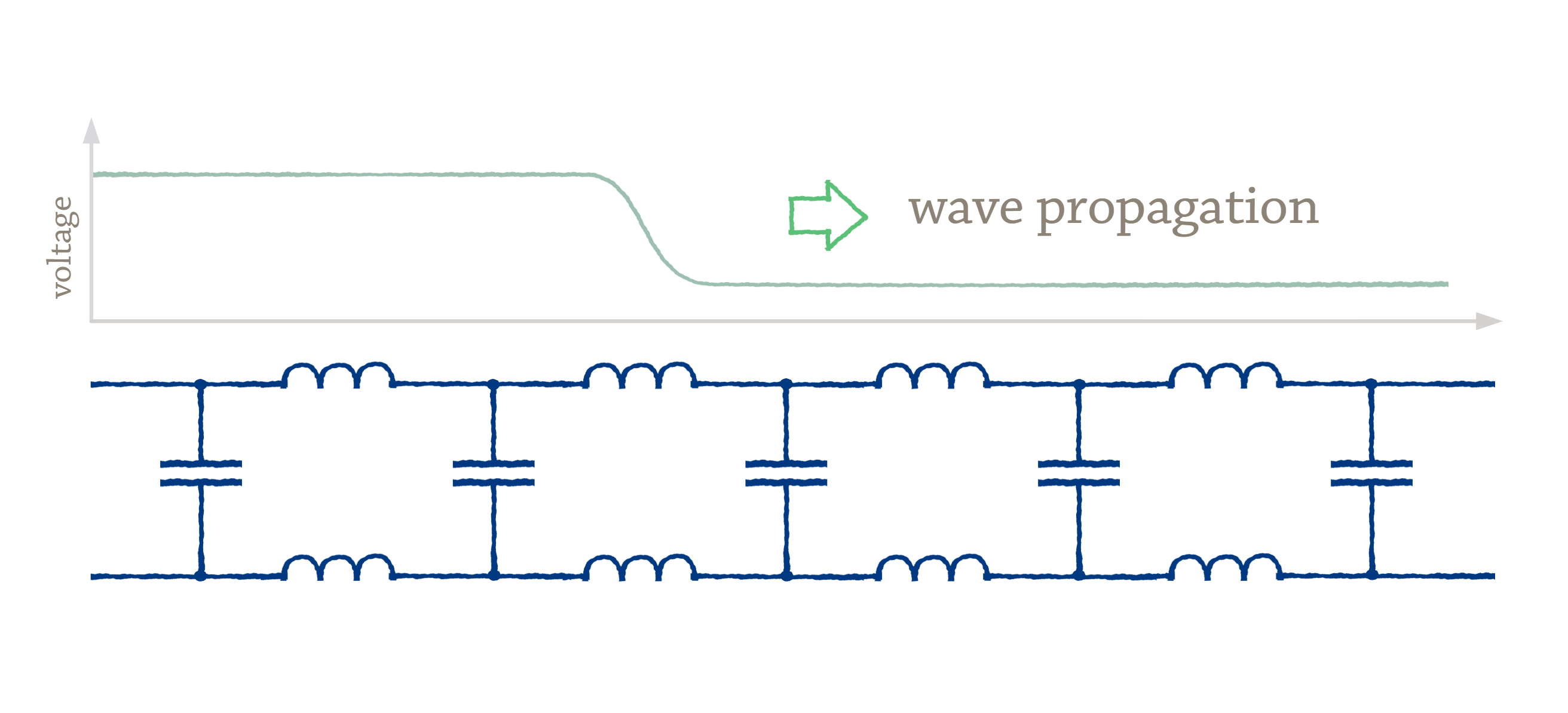
A simple visualization is a model of the coaxial cable as a series of inductances and capacitances that the wavefront needs to interact with on its way from from A to B:
To derive the formula for characteristic impedance, let’s model the conductor’s response to a step voltage increment (Vstep) that traveled x meters down the transmission line. By applying the fundamental formula for signal velocity (vs), we can determine the time needed to reach said point:
The two new values — L/d and C/d — correspond to the transmission line’s inherent inductance and capacitance per some unit of length. The value of d doesn’t need to have any relation to x.
From the discussion of capacitors, we can dust off the formula that relates the voltage applied to a capacitor to the current that must have flowed in a unit of time: I = C × V/t. In our model, the propagating step voltage Vstep is present across x meters of the conductor; the capacitance of this section must be Cstep = C/d × x. We can combine the two formulas to calculate the current that must’ve flowed to get to the expected voltage:
Impedance the ratio between voltage and current; the applied voltage is Vstep and the resulting current is Istep, so we have everything we need to find Z0, too:
Ideally, the characteristic impedance of the transmission line should be matched to the transmitter; that said, a mismatch at the source is less dramatic than a mismatch at the destination. If the characteristic impedance of the cable is too low for the signal source, the transmitter will not be able to build up the desired voltage right away — not until the impedance of the load begins to keep the current in check. Conversely, if the characteristic impedance of the line is too high, the initial current through the load will be lower than it could be.
Most coaxial cables are designed to exhibit characteristic impedance of 50 Ω or 75 Ω; meanwhile, standard traces on a two-layer PCB usually measure around 100 to 150 Ω. To be clear, despite the use of a familiar unit of measurement, this doesn’t mean that the conductor exhibits such resistance to steady currents; it’s simply a way to reason about what happens during signal propagation in a sufficiently long transmission line.
Do I need to care?
That depends. When your signal’s travel time is short in proportion to the its rate of change, the reflections from picoseconds or nanoseconds ago are going to be slight and in-phase with the voltages you’re applying to the wire right now — so the phenomenon has no practical consequences.
For sine waves, the conservative rule of thumb is that if your wire or PCB trace is shorter than one tenth of the wavelength, you don’t need to worry about impedance matching. For signals contained on a small printed circuit board, sine frequencies below 200 MHz should require no special planning. That said, on the upper end, you still need to think about conventional parasitics and RFI.
Of course, there is that gotcha we talked about for square waves: they can be thought of as a sum of sine harmonics, and depending on edge rise times, there might be a fair amount of energy present as high as 11 times the fundamental signal frequency; in other words, a 10 MHz signal might have some properties of a 110 MHz pure-sine wave. This doesn’t always spell trouble — digital signals are meant to withstand a fair amount of distortion — but broadly speaking, some caution is advised at PCB data bus frequencies above 50 MHz, especially if they need to travel to the other end of the board.
When PCB reflections start getting in the way of digital signaling, the usual culprit is a low-impedance source driving a comparatively high-impedance load (e.g., a MOSFET gate). The simplest remedy may be adding a “sink” resistor on the receiving end, connected to the signal’s return path. This is usually paired with a series resistor on the driving side, both to limit peak current and to at least roughly match the characteristic impedance of the trace.
At gigahertz frequencies, the task gets more complicated: the impedance might need to modeled with greater precision and then kept in check with specific board stackups, exotic substrate materials, and the avoidance of vias. That said, at that point, many other convenient circuit design abstractions break down too.
👉 For an explanation of why electronic signals move slower than the speed of light in a vacuum, check out this article. For a catalog of my other articles on electronics, click here.
I write well-researched, original articles about geek culture, electronic circuit design, algorithms, and more. This day and age, it’s increasingly difficult to reach willing readers via social media and search. If you like the content, please subscribe!
Have you seen the stuff at https://antmicro.com/blog/2023/11/open-source-signal-integrity-analysis/ ?
Honestly, still, many, many years later one of the absolute best technical authors we have. Amazing piece.