


Electricity and the speed of light
Does electricity travel at the speed of light?... does light? Yes and no - and you'd be hard-pressed to find an explanation that has an intuitive physical basis.
Back in 2023, I posted an article about signal reflections that opened with a simple, try-it-at-home experiment: we measured the velocity of electronic signals in a run of coaxial cable strewn across the workshop floor. The experiment yielded a figure of 240,000 km/s, or about 80% the speed of light in a vacuum (c).
Yet, the article left one question unanswered: if the signal we’re sending down the wire is just a pattern of alternating electromagnetic fields, why is it moving more slowly than light? More questions arise if we start researching coaxial cables: you can get velocity factors around 90% if you use coax with a core made out of foamed plastic, while solid polyethylene gives you just 65%. Why?
The extinction theorem
First, we should note that light does the same thing: it slows down in matter such as glass. Some online commentators believe it’s because light particles collide with atoms and bounce around; others claim that light is absorbed and then emitted back with a delay. As far as we know, all these theories are wrong.
There is a set of well-known formulas developed in the late 19th century that model this and other behaviors of electromagnetic waves; that said, these formulas tend to deal in the abstract. It’s easy to assert that something must be happening because Maxwell’s equations or Fresnel equations say so; it’s harder to pinpoint the tangible mechanism that makes it true. For the most part, if the equations satisfactorily predict reality, we leave the “why” to philosophers.
For the philosophically-inclined readers, I don’t have a perfect answer, but the most compelling physical model I came across is the Ewald-Oseen extinction theorem. The concept is quite obscure and was formulated for visible light crossing through a homogenous dielectric; that said, it seems to give a credible explanation of why other types of electromagnetic waves could be slowed down by insulators in the vicinity.
To get the ball rolling, let’s assume that all electromagnetic fields always propagate at c. When a simple, approximately-planar waveform is propagating through space, we can take a snapshot in time and visualize the peaks and the valleys of the electric field, like so:

The changing electric field can interact with nearby charged particles. In an insulator, bound electrons can’t move far, but many molecules act somewhat like squish toys: they form electric dipoles that exhibit polarity and can be elastically realigned in response to an external electric field.
To analyze these interactions, let’s consider a signal traveling through a relatively thin slab of insulating material; the location of the sheet is marked by the black vertical line on the illustration below. The electric field aligns the dipoles in the slab in a coherent direction; the dipoles in turn produce a secondary, weaker electric field that radiates away from the surface at the speed of light:
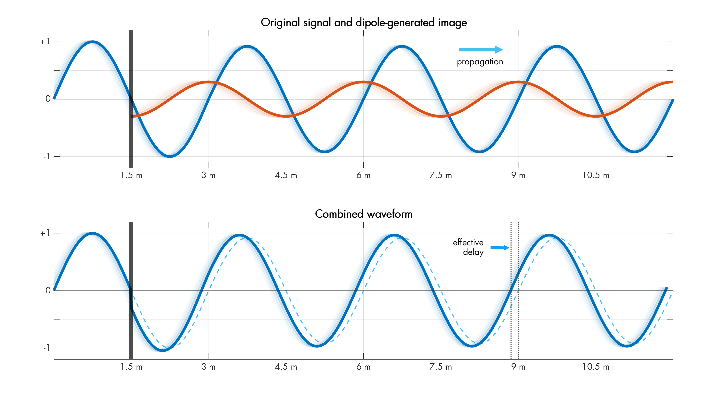
It is easy to intuit that the secondary wave produced by the slab will probably lag in phase compared to the primary signal; this can happen simply because the dipoles don’t react very fast. A rigorous mathematical solution is complicated — but qualitatively, it’s enough to assert that there is some delay, created by some conceivable mechanism.
In one of the earlier posts on the blog, we’ve established that summing two sinusoids of different amplitudes and phases produces another sinusoid with an in-between amplitude and phase. This is what’s happening at the bottom of earlier illustration: the superimposed waveform looks just like the original signal, and is still moving at the speed of light in a vacuum – but when it crossed the slab, it evidently acquired a small delay.
Next, let’s have a look at a scenario with multiple slabs placed along the path of the signal — essentially, a stepwise approximation of a solid. Every time the signal passes through a slab, the interference with the secondary wave adds another delay. If we take a snapshot, the result is a squished sinusoid:

The squished signal has the same frequency as the original but a reduced distance between peaks (i.e., wavelength); the front of the waveform also hasn’t propagated as far as we would have expected. For all intents and purposes, it appears that the signal is traversing the material at a reduced speed.
This is the essence of the Ewald-Oseen extinction theorem; “extinction” refers to the original wave still theoretically being there, but effectively getting replaced with a composite signal that appears to be moving at a speed lower than c. The slowdown is sustained through continued interactions with dipoles, so it goes on only while the wave is moving through the dielectric. The moment the signal exits the medium, it can pick up pace – but can’t make up for the time already lost.
Again, the original model deals with optics, plane waves, and homogenous dielectrics; I don’t think the original math is a drop-in solution for coaxial cables, but at reasonably low frequencies and with transverse waves, I’d wager that the mechanism that produces a reduced signal velocity is functionally similar.
The vs formula
The dipole-based explanation for signal velocity (vs) offers an intuitive basis for the classical but mildly puzzling formula that ties that velocity to a pair of physical parameters known as magnetic permeability (μ) and electric permittivity (ε):
These parameters may seem alien, but they’re strongly affected by the presence of electric and magnetic dipoles and directly tied to the electronic concepts of capacitance (C) and inductance (L) per unit length (d). This allows the equation for an idealized (long) conductor to be expressed the following way:
We typically talk of inductance and capacitance as properties of specific electronic components, but every sufficiently long line can be described as having a series inductance that opposes the change in current, along with a conductor-to-conductor capacitance that requires a non-zero current to flow before the voltage goes up. Without these effects, signal propagation would always be effortless and instantaneous. That would be incompatible not only with common sense, but also with the theory of relativity.
An interesting corollary of this last remark is that although the actual values of L and C are most commonly associated with matter, vacuum necessarily has a non-zero impedance and capacitance too; the numbers, when plugged in the aforementioned formula, work out to a signal propagation speed of vs = c.
In the formula, both L and C must be specified per unit of length (d). To circle back to the earlier experiment, quality coax might have an inductance of around 210 nH/m and a capacitance of 80 pF/m. After a bit of unit-wrangling, the equation yields:
And now, we more or less know what kind of sorcery this is.
👉 For more articles on physics, click here, here, here, or here.
I write well-researched, original articles about geek culture, electronic circuit design, and more. If you like the content, please subscribe. It’s increasingly difficult to stay in touch with readers via social media; my typical post on X is shown to less than 5% of my followers and gets a ~0.2% clickthrough rate.
Love your stuff.
Good discussion