Core concepts #2: impedance is complex

Modeling impedance in two dimensions, RC / RL / LC circuits, and why an LCR meter is not quite what it seems.

In a recent introductory article on electronics, I talked about impedance (Z): the tendency for components and circuits to resist the flow of current. The phenomenon has three constituent parts: resistance, capacitive reactance, and inductive reactance. Superficially, all of these effects look like resistance and express the same relationship: the ratio of the applied voltage to the current flowing through the device.

The question we haven’t answered in the earlier article is how to deal with situations where an inductor, a capacitor, and a resistor are strung together in some fashion. The answer is easy to find online, but you’d be hard-pressed to find a source that actually explains why the rules are what they are.

In this article, we’ll answer the why by having a look at two specific examples: a series LC circuit and a series RC / RL one.

A quick recap: R, X_C, X_L

Let’s start with a couple of definitions from the earlier article. Of the three concepts that add up to impedance, resistance (R) is the easiest to grasp. It’s a phenomenon somewhat similar to aerodynamic drag. It’s commonly associated with heat dissipation in resistors, semiconductors, and long runs of wire. Formally, the value of R is equal to V/I — i.e., the ratio of the applied voltage to the current it is capable of inducing through a given resistor.

Capacitive reactance describes the same relationship between current and voltage, but it typically has to do with the reversible storage of potential energy in electric fields. The concept is valid only for sinusoidal waveforms; its magnitude changes with the frequency of the driving signal. For a given sine frequency (f) and a known capacitor value (C), we’ve previously derived the following formula:

\(X_C = {1 \over {2 \pi f C}}\)

In essence, this says that the the current induced by a given sinusoidal voltage waveform is proportional to f and C. The 2π constant is a matter of the mathematical convention to define sin(x) over radians, resulting in a relationship of 2π = 1 Hz; a more thorough explanation can be found in the article linked in the intro to this post.

Finally, inductive reactance generally has to do with the creation of magnetic fields inside an inductor, in a manner fairly similar to the kinetic energy of a moving mass. The effect is also sine-wave-specific and frequency-dependent. For a given signal frequency and an inductor value (L), its magnitude in ohms is expressed as:

\(X_L = 2 \pi f L\)

In other words, the current increases in inverse proportion to f and L, with the now-familiar 2π bit thrown in.

L-C in series

In the earlier article, we observed (and then proved) that the sinusoidal voltage across the terminals of a capacitor lagged one fourth of the period in relation to applied current. If we describe current with a sine function, it would mean that to calculate the voltage waveform, we’d need to offset the voltage timing expression by -90°:

\(\begin{array}{c} I(x) = I_{peak} \cdot sin(x) \\ V(x) = V_{peak} \cdot sin(x -90^\circ) \\ \end{array}\)

For an inductor, the shift would be equal to +90°.

In circuit analysis, we often start with voltages and then look at currents, but in this instance, we actually need to look at it the other way round. In the case of an inductor and a capacitor connected in series, the current flowing through the components must be the same; what comes in must come out, and there’s no place for electrons to chill. In other words, it’s not the currents but the voltages across the components’ terminals that get out of sync. The question then becomes: given a particular driving current, how will the out-of-phase voltages interact?

To get going, we can note that each component has a fixed reactance at a given frequency, so the unknown but linear combination of these reactances should also be const. In other words, if the applied voltage is a sinusoid, the current will also have this property.

A general, simplified equation for that current might be written as:

\(I(x) = I_{peak} \cdot sin(x)\)

Again, we don’t know the combined impedance, so we don’t know the value of I_peak — but we can make progress without that. At this point, we also don’t care about the frequency or phase of the current, because we’re not trying to relate it to anything else. We can treat it as a pure sinusoid described by some timing expression x.

Fundamentally, capacitive and inductive reactances both describe the same relationship between voltage and current: V_peak / I_peak. Keeping this in mind, we can construct a pair of waveforms for the appropriately phase-shifted voltages that are bound to appear across the terminals of the inductor and the capacitor:

\(\begin{alignat*}{3} V_L(x) &= X_L &&\cdot I_{peak} \cdot \underbrace{sin(x + 90^\circ)}_{\textrm{same as } cos(x)} &&= +X_L \cdot I_{peak} \cdot cos(x) \\ \\ V_C(x) &= X_C &&\cdot I_{peak} \cdot \underbrace{sin(x - 90^\circ)}_{\textrm{same as } -cos(x)} &&= -X_C \cdot I_{peak} \cdot cos(x) \end{alignat*} \)

We model how the voltages are offset from the input current — but again, we don’t care about the absolute phase or frequency of the current. We just need to describe the relative shift.

Voltages in series sum in a straightforward way — two 1.5 V batteries add up to 3 V. That is to say, the overall voltage across the L-C pair is:

\(V_{LC \textrm{ (series)}}(x) = V_L(x) + V_C(x) = (X_L - X_C) \cdot I_{peak} \cdot cos(x)\)

This tells us that in this setup, the effects of X_L and X_C don’t add constructively; instead, they subtract. The peak voltage is given by the multiplier in front of cos(x) — the trigonometric function itself maxes out at 1 — so:

\(\begin{array}{c} V_{peak} = (X_L - X_C) \cdot I_{peak} \\ Z_{LC \textrm{ (series)}} = {V_{peak} \over I_{peak}} = {(X_L - X_C) \cdot \cancel{I_{peak}} \over \cancel{I_{peak}}} \\ \\ \textrm{Solution: } Z_{LC \textrm{ (series)}} = X_L - X_C \end{array}\)

When we plot any functions that describe the attenuation or amplification of signals, we usually rely on a logarithmic (log-log) scale. The scale is uniquely suited for the task: a 10× increase is always represented by the same distance on the plot, no matter if the starting value is 1, 10, or 100. A sample log-log plot of the absolute value of Z_{LC (series)} across a range of signal frequencies is shown below:

The behavior of a series LC circuit for C = 100 µF, L = 1 mH.

On this graph, impedance is dominated by the effects of the capacitor all the way to around 100 Hz. We can see that the curve clings on to the dashed line representing X_C = 1/(2πfC). Later on, at several kilohertz, inductive reactance takes over. From that point on, the curve follows the X_L = 2πfL line and the capacitor has almost no say.

Around 500 Hz, there’s also a pronounced dip where the value of Z_{LC (series)} apparently drops to zero. This is where the value of X_L is equal to the value of X_C.; the voltage developing across the capacitor is the same as the voltage across the inductor, except it has the opposite sign. This nets out to zero volts, so the flow of (perfectly sinusoidal) current is not impeded in any way.

We can find this resonant frequency in a pretty simple way:

\(\begin{align*} \textrm{Assumption} &: X_L = X_C \\ \textrm{Formulas expanded} &: {2 \pi f \, L} = {1 \over 2 \pi f \, C} \\ \textrm{Moving } f \textrm{ to the left} &: f^2 = {1 \over 4 \pi^2 \cdot C \cdot L} \\ \textrm{Final expression} &: f = {1 \over 2 \pi \sqrt{LC}} \end{align*}\)

Of course, in practice, the “infinite current” singularity doesn’t happen. If the current is gracefully limited by the series resistance of the signal source or the internal resistance of the inductor / resistor, you essentially get an RLC circuit where the resonance peak is “softened” in relation to the value of R.

R-L and R-C in series

The math gets a bit more complicated if we throw a resistor into the mix. Resistance contributes no phase shift, so what comes in as a sin(x) also comes out as a sin(x). This is halfway between the effects of capacitance and inductance, so we can safely guess that the calculation of the combined effect won’t be a simple matter of subtracting two values.

To get going, we can start with a model of voltages for a series RL circuit. Similarly to what we did in the previous section, we assume a current modeled by sin(x). Again, the resistance has no phase shift, while the inductance has a +90° shift that turns it into cos(x):

\(\begin{alignat*}{2} V_L(x) &= X_L &&\cdot I_{peak} \cdot cos(x) \\ V_R(x) &= R &&\cdot I_{peak} \cdot sin(x) \end{alignat*}\)

We can try to solve for the sum of voltages manifesting across the terminals – but this time, the answer won’t be obvious:

\(V_{RL \textrm{ (series)}}(x) = V_L(x) + V_R(x) = I_{peak} \cdot (R \cdot sin(x) + X_L \cdot cos(x))\)

No matter how we slice and dice it, we have no trivial way to group R and X_L vis-a-vis a common timing function to build an equation for impedance.

Again, most online tutorials just pull the impedance formula for this scenario out of thin air. But a pretty neat trigonometric solution is shown below:

Elements of a visual solution to A · sin(x) + B · cos(x).

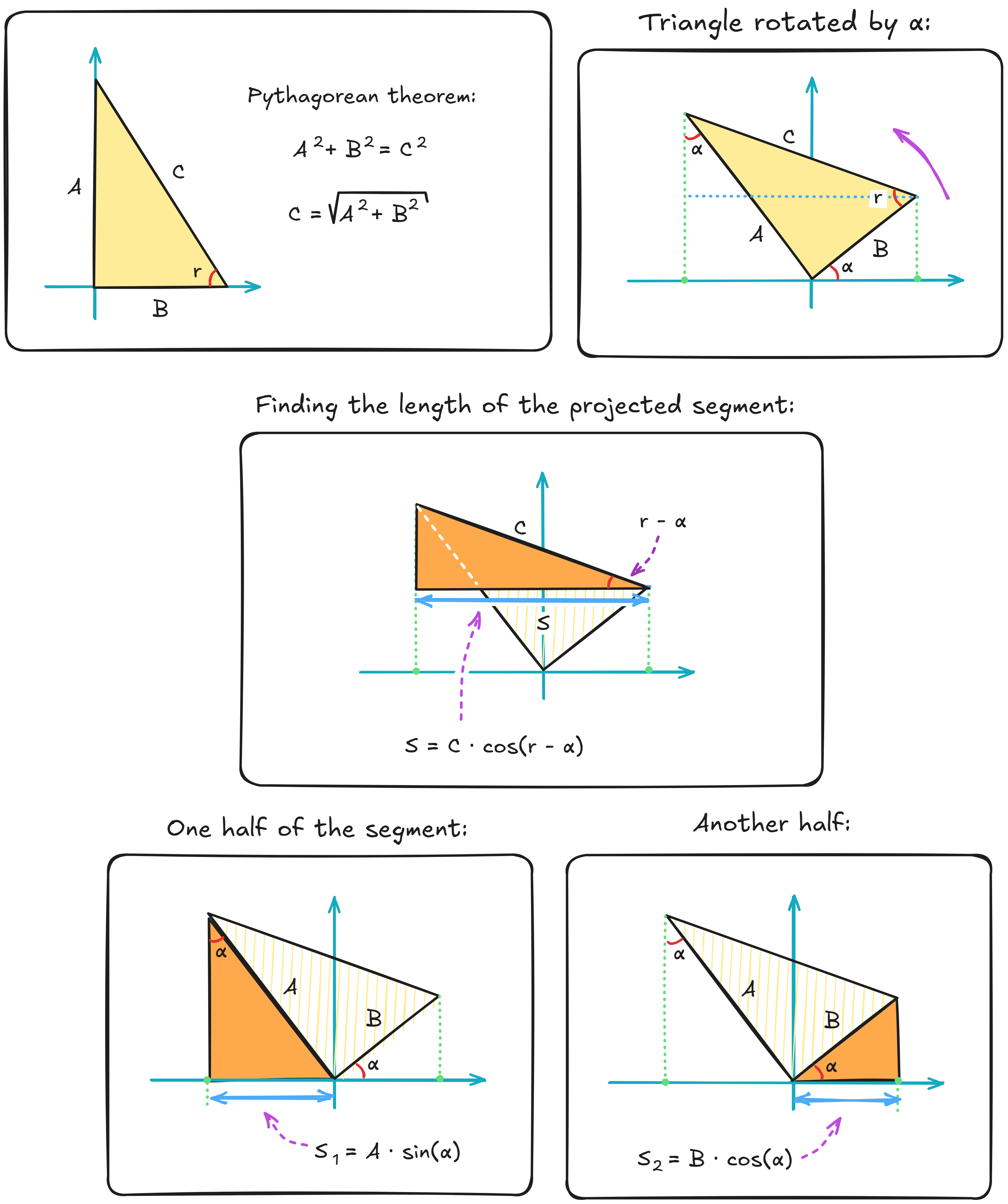
We start by drawing a right-angled triangle. The triangle has one three sides labeled A, B, and C – the last one being the hypotenuse. It also features an angle, r, which is dictated by the ratio of A to B, but we don’t need to solve that.

Next, we rotate the triangle counterclockwise by α and then draw a projection of the now-tilted hypotenuse onto the horizontal axis. We call this projected segment S. We can easily calculate its length using the helper triangle added in the middle panel. The length works out to C · cos(r – α).

In the last two panels, we calculate the length of S in an alternative way: as a sum of two sub-segments, S₁ and S₂. With the aid of two helper triangles, we can easily establish that S₁ equals to A · sin(α) and that S₂ comes out to B · cos(α). This lets us write the following equality:

\(\begin{align*} S_1 + S_2 &= S \\ A \cdot sin(\alpha) + B \cdot cos(\alpha) &= C \cdot cos(r - \alpha) \end{align*}\)

Further, by applying the Pythagorean theorem to the starting triangle, we can obviously establish that C = √(A² + B²). So, another way to express the solution is:

\(A \cdot sin(\alpha) + B \cdot cos(\alpha) = \sqrt{A^2 + B^2}\cdot cos(r - \alpha)\)

This is a remarkable result, because it tells us that a sum of sin(…) and cos(…) waves of different amplitudes (A and B) but the same timing variable (α) can be expressed as another sine wave of the same frequency but with some fixed shift (r).

Again, we could try finding r, but that’s unnecessary unless we want to solve for the voltage phase offset. For finding out the magnitude of impedance, we have all we need to rewrite the voltage equation into a “good enough” form of:

\(V_{RL \textrm{ (series)}}(x) = \sqrt{R^2 + {X_L}^2} \cdot I_{peak} \cdot cos(\textrm{<something>})\)

This lets us write the impedance solution for a series RL or RC circuit:

\(Z_{RL,RC \textrm{ (series)}} = \sqrt{R^{\,2} + {X_{L,C}}^2}\)

The plot of this formula across a range of frequencies is less exciting than the LC case. There’s no resonant dip, just a smooth transition between the horizontal line corresponding to constant resistance, and a slope corresponding to the behavior of a capacitor or an inductor:

The behavior of a series RC circuit for R = 10 kΩ, C = 1 µF.

The crossover frequency can be derived analogously to what we did for the LC case; the RC result is:

\(f = {1 \over 2 \pi R C}\)

A more interesting observation is that a bit out of the blue, the Z_RC / Z_RL equation that we came up with just moments ago is awfully similar to the Pythagorean theorem. We can write it down as:

\(Z^2 = R^2 + X^2\)

We have previously established that capacitive and inductive reactances subtract. This new rule tells us that Z (or less ambiguously, |Z| — more about that soon) is the same as the length of a diagonal of a rectangle on a Cartesian plane if the rectangle’s width and height are described by R and X:

Converting a |Z| and θ measurement into R and X_L readings.

Meanwhile, the resulting phase shift is just the angle under the diagonal; it would be 0° for a purely-resistive impedance, 90° for a purely-inductive one, or an intermediate value if we’re dealing with a mix of these effects.

It’s worth noting that the proof isn’t specifically about impedances; it’s about the effects of mixing sine waves that are offset one-fourth of a cycle in phase. In effect, this interpretation works for any sine-related quantities spaced 90° apart. We can use it for currents, voltages, and more exotic phenomena. But for now, we’re still sticking to impedance.

More fun with Cartesian coordinates

The new interpretation allows us to breeze through various problems because it lets us translate between R, X, |Z|, and phase shifts with ease. For example, if we observe a signal with a measured magnitude of impedance of |Z| and a voltage-vs-current phase shift of θ, we can easily figure out the equivalent values of R and X_L or X_C that produce this shift:

\(\begin{array}{ccc} R = |Z| \cdot cos(\theta) \\ X = |Z| \cdot sin(\theta) \end{array}\)

That might lend itself to a characterization of some component under test, or give us an abstract R-C-L equivalent of a more complex linear circuit.

In the same vein, the two-dimensional interpretation of impedance gives us a simple way to look at a schematic and determine phase shift between the current flowing through and the resulting voltage. The tangent function describes the ratio of the opposite (X) to the adjacent (R) in the right-angled triangle under the impedance vector, so if we know the X and R values, we can just calculate:

\(tan(\theta) = {X \over R}\)

To get from the ratio to an angle, we lean on the inverse of tan — arctan:

\(\theta = arctan({X \over R})\)

To illustrate the use of these formulas, let’s take the series RC case. In this case, X = -X_C = -1/(2πfC), so the angle formula works out to:

\(\theta_{RC\ (series)} = -arctan({1 \over 2 \pi f RC})\)

Again, the result in radians. The series series RL solution is:

\(\theta_{RL\ (series)} = arctan({2 \pi L \over R})\)

Calculator apps usually output the value in radians, so you need to multiply the result by 360°/(2π) — aka 180°/π — to get the value in degrees.

Again, what we’re describing here are strictly the phase shifts between voltage and current: +90° would mean that the voltage appears to be lagging behind current, while -90° would mean that it’s ahead. RC circuits are also used for other purposes, and in these contexts, we might be looking at voltage-to-voltage shifts at the circuit’s midpoint. The rules for that are a bit different.

Translating between R, X, Z, and θ aside, the Cartesian model also makes it easy to sum multiple impedances while keeping track of overall phase shifts. For example, if we apply a voltage across two series impedances — |Z₁| with a phase of θ₁ and |Z₂| with a phase of θ₂ — the combined impedance can be calculated by first splitting the impedances into the R and X components, and then summing these distances the standard way:

\(\begin{array}{ccc} R_{1,2} = |Z_{1,2}| \cdot cos(\theta_{1,2}) \\ X_{1,2} = |Z_{1,2}| \cdot sin(\theta_{1,2}) \\ R_{total} = R_1 + R_2 \\ X_{total} = X_1 + X_2 \\ \end{array} \)

With this done, we can recompute the magnitude of summed impedance from the Pythagorean theorem, and find the new phase angle using arctan(…):

\(\begin{array}{c} |Z_{total}| = \sqrt{{R_{total}}^2+{X_{total}}^2} \\ \theta_{total} = arctan({X_{total} \over R_{total}}) \end{array} \)

In the end, impedance is complex

In practice, it gets cumbersome to use |Z| and θ as the representation of impedance when doing more complex circuit math when we constantly need to convert to R and X behind the scenes to recompute the values.

Instead, we can stick to R and X as the basis of all the intermediate math, converting to magnitude and phase only when we absolutely need it (typically, as the final step).

Further, instead of two independent variables, we can keep track or Z as a “vector quantity” — that is, a pair of coupled numbers, essentially the Cartesian (x, y) coordinates that describe the size of the two-dimensional impedance arrow from our earlier model:

\(Z = (R, X) \)

We can define intuitive arithmetic rules for working with these “composite” values, mimicking standard geometry. For example, for adding two impedances, the rule would be:

\((x_1, \ y_1) + (x_2, \ y_2) = (x_1 + x_2, \ y_1 + y_2) \)

Similarly, multiplication by a number would just scale the vector, like so:

\(a \cdot (x, \ y) = (a \cdot x, \ a \cdot \ y) \)

Subtraction and division work essentially the same way.

In EE literature, impedance is often treated as such a vector; this is why at some point in the article, to avoid ambiguity, I started referring to the scalar magnitude of impedance (the length of the arrow) as |Z|. That said, instead of Cartesian (x, y) pairs, electrical engineers usually keep the values at an arm’s length using complex numbers.

Don’t panic! Complex numbers are actually not that complex. They’re constructed out of a “real” part and an “imaginary” part; the latter is always multiplied by a magic-bean value of j = √-1 that keeps the terms separable:

\(Z = R + j X\)

This might sound confusing, but it’s not hugely different to inventing a special value of 🐱, with the rule that 🐱 is not a normal number, so you can’t commingle the terms that contain a 🐱 with the ones that do not:

\(\underbrace{(1 + 2🐱)}_\textrm{cat-complex 1} + \underbrace{(3 + 10🐱)}_\textrm{cat-complex 2} = \underbrace{\underbrace{(1+3)\vphantom{🐱}}_{\textrm{non-cat count}} + \underbrace{(2+10)\vphantom{🐱}}_\textrm{cat count}🐱}_\textrm{cat-complex result}\)

We can sum the cat and non-cat expressions individually, so the simplified result of this addition is a cat-complex number of 4 + 12🐱. In the same vein, when summing impedances that consist of a “real” R part and a j-coupled X part, you’d do the following math:

\(Z_{total} = Z_1 + Z_2 = \underbrace{\underbrace{(R_1 + R_2)}_\textrm{real part} + j \underbrace{(X_1 + X_2)}_\textrm{imaginary part}}_{\textrm{complex result: } Z_1 + Z_2}\)

Most of the time, j isn’t doing anything of note; it’s there just to keep the terms separate. If something is multiplied or divided by it, it’s stuck in the imaginary realm and can’t be commingled with any of the real terms.

To be fair, there is a fairly important rule that applies to j and not to cats: j² = -1 (🐱² = ???). This might seem like a defect in the abstraction, but it’s actually what makes j well-suited for Cartesian coordinates and other “orthogonal” quantities; for a discussion of why we want this to happen, you can check out this followup article.

We could work with a 🐱-based system without this behavior, but this just means that we’d sometimes end up with terms containing two cats (🐱🐱). We’d then need to decide what that means. Since one cat represented a sine wave offset by 90°, we’d inevitably have to conclude that two cats correspond to a 180° shift — and just subtract these terms from the catless (0°) part. In the j-based system, j · j = -1, so this subtraction happens automatically.

In some contexts, you can also see a mysterious entity called s. There is a more complex mathematical backstory to this symbol, but when we’re talking about steady sinusoidal signals in linear circuits, s can be thought of simply as a shorthand that combines j with the common frequency expression of X_L and X_C equations: s = j·2πf. This lets you write the complex impedance of an inductor in series with a resistor as:

\(Z_\textrm{LC (series)} = R + sL \)

The case of an capacitor in series with a resistor is:

\(Z_\textrm{RC (series)} = R + \frac{1}{sC}\)

Again, in these contexts, the appearance of s is just a shorthand that saves you a bit of typing, and not a sign of any particularly advanced math.

The multimeter conundrum

Now that we have the relationship between R and X figured out, let’s talk about digital multimeters (DMMs). You can use a DMM to characterize resistors, capacitors, and inductors — but how does that work, and how much you can trust the number shown on the screen?

Well, resistors are a simple special case: the meter can apply a small DC voltage to the terminals of the device under test, indirectly measure the resulting current (usually by observing the voltage drop across a precision shunt placed in series), and then calculate the magnitude of impedance (|Z| = V/I).

A real-world resistor exhibits some parasitic inductance in the conductive path, along with parallel capacitance due to the presence of a less-conductive layer sandwiched between two metal terminals:

Modeling a real-world resistor.

That said, at f ≈ 0 Hz, inductive reactance of the component’s conductive path is about zero, while the parallel capacitive reactance is so high that the “side” path via the parasitic capacitor can be ignored. In other words, when characterizing resistors at DC, |Z| can be assumed to be equal to R.

The measurement of capacitors also involves measuring impedance — but this time, it’s done with an alternating current. The resulting value is some combination of R, X_C, and X_L. That said, because capacitors usually have very low parasitic resistance (ESR), it’s often assumed that R = 0; at low signal frequencies — below 100 kHz or so — the component’s X_L is usually also negligible. Under these circumstances, the meter can roughly assume that |Z| = X_C and then use the capacitive reactance formula — X_C = 1/(2πfC) — to solve for C to arrive at a ballpark farad figure to put on the screen.

In principle, the same approach could be followed for inductors. That said, relatively few DMMs offer this mode; this is in part because discrete inductors are less common in modern circuits, but also because small inductors often exhibit quite a bit of wire resistance — possibly as high tens or hundreds of ohms. Under such circumstances, assuming that R = 0 would taint the readings more than it does for most capacitors.

This is where LCR meters come into play. On the face of it, the meter looks like a nerfed DMM, only capable of measuring inductance (L), capacitance (C), and resistance (R). One has to wonder how this piece of gear survived this long, and why it commands a considerable premium for such a limited feature set.

The answer is that the “LCR” moniker is a bit of a misnomer. A better name might be a “|Z|θ meter”. The first thing the meter does is measuring the magnitude of impedance at a user-specified signal frequency. It does so by outputting an AC signal, comparing the observed voltage amplitude and current, and then calculating |Z| = Vpeak/Ipeak. Just like in a DMM, the measurement represents the combined effect of resistive, capacitive, and inductive effects; it tells us nothing about the exact values of L, C, or R.

That said, the other parameter the meter computes with high accuracy is the phase offset between the voltage and current (θ) — and that extra bit of information changes everything. As discussed earlier, if we know the length of the impedance vector and the phase angle, we can get back to the values of R and X_L or X_C:

\(\begin{array}{ccc} R = |Z| \cdot cos(\theta) \\ X = |Z| \cdot sin(\theta) \end{array}\)

And that’s precisely the math that an LCR meter does to split the |Z| and θ measurements into reactance and resistance. The resistance value is reported as-is; the reactance is converted into C or L by working back from the standard formulas:

\(\begin{align} X_{C} = {1 \over 2 \pi f C} \quad &\rightarrow \quad C = {1 \over 2 \pi f X_C} \\ X_{L} = {2 \pi f L} \quad &\rightarrow \quad L = {X_L \over 2 \pi f} \end{align}\)

So… why aren’t all meters doing that?

Now that we know that these devices are actually |Z|θ meters, we can talk about the unexpected usability problems that arise if one tries to use them to measure R, C, and L values without understanding the underlying math.

To illustrate, if you take a 10 µF multilayer ceramic capacitor, connect it to an LCR meter, and set the test frequency to 200 kHz, you might end up with a reading that looks quite a bit off. It might be tempting to blame it on the capacitor, but MLCCs are supposed to behave properly well into tens of megahertz. So, what’s going on?

The answer has to do with the measurement the meter is actually trying to make: scalar impedance. For an MLCC operated at 200 kHz, this comprises almost entirely of its capacitive reactance, which is — again — given by the following formula:

\(X_C = {1 \over {2 \pi f C}}\)

If we plug in f = 200 kHz and C = 10 µF, X_C works out to about 80 mΩ; that’s too low for many meters to measure accurately. If you lower the frequency to 1 kHz, the math works out to 16 Ω — a much more reasonable result. The issue would be evident when looking at the raw |Z| reading, but it’s easy to miss if you’re staring at the computed C value instead.

There is an inverse problem at low frequencies: a 10 pF capacitor tested at 100 Hz shows up as an impedance of 160 MΩ. Switching to 50 kHz puts the impedance at several hundred kΩ, which is much easier to deal with. Either way, LCR meters are not nearly as plug-and-play as they might seem.

All this added nuance is part of the reason why DMMs almost always resort to the “dumber” but more bulletproof way of making these measurements.

Do I need an LCR meter on my workbench?

Unlike an oscilloscope or a DMM, an LCR meter is not essential in most hobby workshops. The device tends to come in handy when working with analog circuits, especially in the audio and RF domain; it’s also useful for troubleshooting inductors of all shapes and sizes, and for weeding out electrolytic caps that have gone bad. On the flip side, if you’re working mainly in the digital domain, the meter is likely to end up collecting dust.

It’s perhaps worth noting that for casual experimentation where precise impedance readings are unnecessary, an oscilloscope working in tandem with a signal generator can offer comparable insights — possibly across a wider range of frequencies.

Addendum: parallel circuits

Before the meter segue, we talked about series LC, RC, and RL circuits; the extension to a series RLC layout is also trivial: it’s just a matter of calculating X = X_L - X_C, and then Z_{RLC (series)} = √(R² + X²).

But what about parallel arrangements? There is a well-known formula for summing parallel resistances, but it’s one of these things that are often taught without proper explanation — so let’s try to fix that.

When we have two parallel resistances, there are two independent currents through two branches of the circuit; that said, the voltage across the parallel section must be common to both paths, because the components’ respective terminals are shorted with each other. This is essentially the inverse of the series scenario, where the voltages could differ but the current had to remain the same.

If there’s a given voltage-based signal applied to the parallel circuit, how do we go about calculating per-branch currents? From Ohm’s law, the rated value of each resistor is R = V/I; rearranging this for current, we get I = V/R, so:

\(\begin{array}{c} I_{R1} = {1 \over R1} \cdot V \\ I_{R2} = {1 \over R2} \cdot V \\ I_{total} = I_{R1} + I_{R2} = ({1 \over R1} + {1 \over R2}) \cdot V \end{array} \)

If we know the sum of currents, we can calculate the equivalent resistance of both branches, too:

\(R_{total} = {V \over I_{total}} = {\cancel{V} \over ({1 \over R1} + {1 \over R2}) \cdot \cancel{V}} = {1 \over {1 \over R1} + {1 \over R2}}\)

So, it’s a reciprocal of the sum of reciprocals.

The relationship between series and parallel formulas for LC, RL, and RC is similar. For example, for parallel RC, you get:

\(Z_{RC \textrm{ (parallel)}} = {1 \over \sqrt{{1 \over R^2} + {1 \over {X_C}^2}}}\)

Because the notation is somewhat tedious, we often use a special symbol — two vertical lines (‖) — to denote the addition of parallel impedances. The following notations are equivalent:

\(R1 \ \Vert \ R2 = {1 \over \frac{1}{R1} + \frac{1}{R2}}\)

👉 To continue reading about capacitors as signal filters, check out this write-up. For a demo of how to use complex numbers to figure out the attenuation of a two-stage RC filter, see here. For more articles about electronics, click here.

---

I write well-researched, original articles about geek culture, electronic circuit design, and more. If you like the content, please subscribe. It’s increasingly difficult to stay in touch with readers via social media; my typical post on X is shown to less than 5% of my followers and gets a ~0.2% clickthrough rate.