


Square waves, or non-elephant biology
How to think about non-sine waveforms if all the electronic theory deals in sines?
For newcomers, it’s easy to conclude that there’s something rotten in the kingdom of electronics: virtually all the intuitive, hobbyist-friendly rules for analyzing the response of electronic circuits work only for sine waves. The underlying theory dates back to the early days of radio; although sine waves crop up often in nature, the math doesn’t seem to be applicable to, say the world of square waves in modern digital circuitry.
The fixation of sine waves makes some sense. As discussed in an earlier introductory article, such waveforms have some nice mathematical properties: when they travel through capacitors or inductors, they emerge on the other end looking essentially the same, with their amplitude and phase adjusted according to a simple formula. The case of other waveforms is more complex and notionally calls for advanced calculus.

Still, the explanation feels like a cop-out. In effect, we have divided the field into elephant and non-elephant biology — and we’re really proud that the elephant stuff is quite easy to grasp!
Luckily, there’s one invaluable and accessible trick for dealing with non-elephant square waves: as it turns out, they can be approximated as a sum of a sine wave at the fundamental frequency, plus sine waves at that frequency’s odd multiples. Specifically, the time-domain formula is:
Alternatively, a more straightforward notation is:
Although the sum is notionally infinite, the cool part is that the sequence quickly converges to the expected waveform. The following plots show the first couple of approximations for sum lengths of 1, 2, 6, and 20:
If you have gnuplot installed, you can experiment with this convergence using the following set of commands:
set samples 2000
odd_h(x, n) = sin(x * (2*n - 1)) / (2*n - 1)
plot sum [n=1:20] 4/pi * odd_h(x, n)
Replace “20” in the last line with the number of odd frequency multiples you wish to sum.
As should be evident from the illustration, by the time you get to n = 6 (fundamental frequency times 11), the waveform looks close enough to the real deal for almost all intents and purposes; at that point, the average approximation error is less than 10%, and the rising and falling edges are within 3° of vertical. The inclusion of further multiples (“harmonics”) offers diminishing returns as a consequence of the increasing divisor in the underlying expression.
You can also approach this the other way round. The fast Fourier transform (FFT) is an important mathematical tool that deconstructs complex signals into a spectral view of sine wave frequencies. Using an oscilloscope to apply FFT to a real-world 1 MHz square wave yields the following plot:
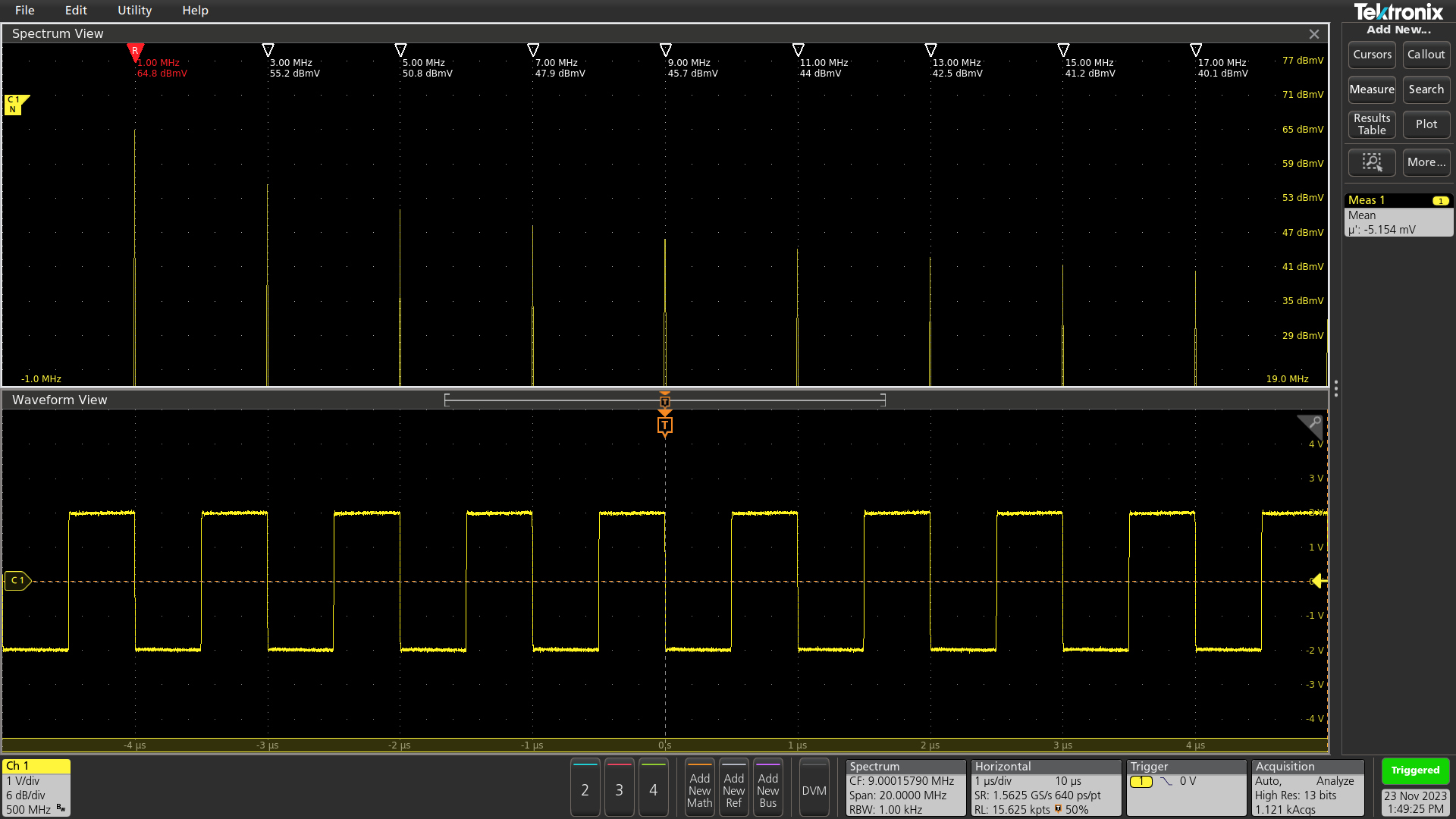
The vertical scale of the spectrum plot is logarithmic; the gradations are 6 dB apart, which is a needlessly complicated way for electrical engineers to say that each line corresponds to a 2× change in signal amplitude. You can clearly see that the fundamental frequency is followed by a series of peaks at odd harmonics (3×, 5×, 7×, etc). The second peak has an amplitude of about 1/3rd of the fundamental frequency (a difference of 9.6 dB); the third one is about 1/5th; and so forth. The sixth spike at 11 MHz has an amplitude of just about 9% of the first one (-20.8 dB).
The ability to deconstruct square waves into a finite (and short!) sum of sine harmonics is surprisingly useful. For example, the approach allows you to intuitively explore the behavior of lowpass, highpass, or bandpass filters that attenuate and phase-shift some of these harmonics depending on their frequency. All you have to do is compute a new sum of a handful of appropriately-adjusted constituent waveforms.
To illustrate the qualitative worth of this approach, we can also revisit the topic of decoupling capacitors from an earlier article. We now know that a 10 MHz square wave with brisk (sub-10%) rise and fall times can be roughly modeled as a series of significant sine harmonics extending to about 110 MHz. This explains the difficulty of fully suppressing digital switching noise with a single capacitor: as discussed in that article, in the vicinity of 100 MHz, parasitic inductive characteristics of low-cost MLCCs become quite pronounced and significantly limit the current such a capacitor can source. By the time you get to 200 MHz, the components do very little decoupling at all.
👉 For the sine-wave representation of more complex signals, check out the article on DFT. For an explanation of why sine waves are common in physics, click here. For more on analog and digital electronics, please visit this index page.
I write well-researched, original articles about geek culture, electronic circuit design, and more. If you like the content, please subscribe. It’s increasingly difficult to stay in touch with readers via social media; my typical post on X is shown to less than 5% of my followers and gets a ~0.2% clickthrough rate.