Radios, how do they work?

A brief introduction to antennas, superheterodyne receivers, and signal modulation schemes.

Radio communications play a key role in modern electronics, but to a hobbyist, the underlying theory is hard to parse. We get the general idea, of course: we know about frequencies and can probably explain the difference between amplitude modulation and frequency modulation. Yet, most of us find it difficult to articulate what makes a good antenna, or how a receiver can tune in to a specific frequency and ignore everything else.

In today’s article, I’m hoping to provide an introduction to radio that’s free of ham jargon and advanced math. To do so, I’m leaning on the concepts discussed in three earlier articles on this blog:

• Core concepts in electronic circuits,

• Signal propagation delays and signal reflections,

• Frequency domain analysis with DFT and DCT.

If you’re rusty on any of the above, I recommend jogging your memory first.

Let’s build an antenna

If you’re familiar with the basics of electronics, a simple way to learn about antennas is to imagine a charged capacitor that’s being pulled apart until its internal electric field spills into the surrounding space. This would be a feat of strength, but bear with me for a while:

Turning a capacitor into a terrible antenna.

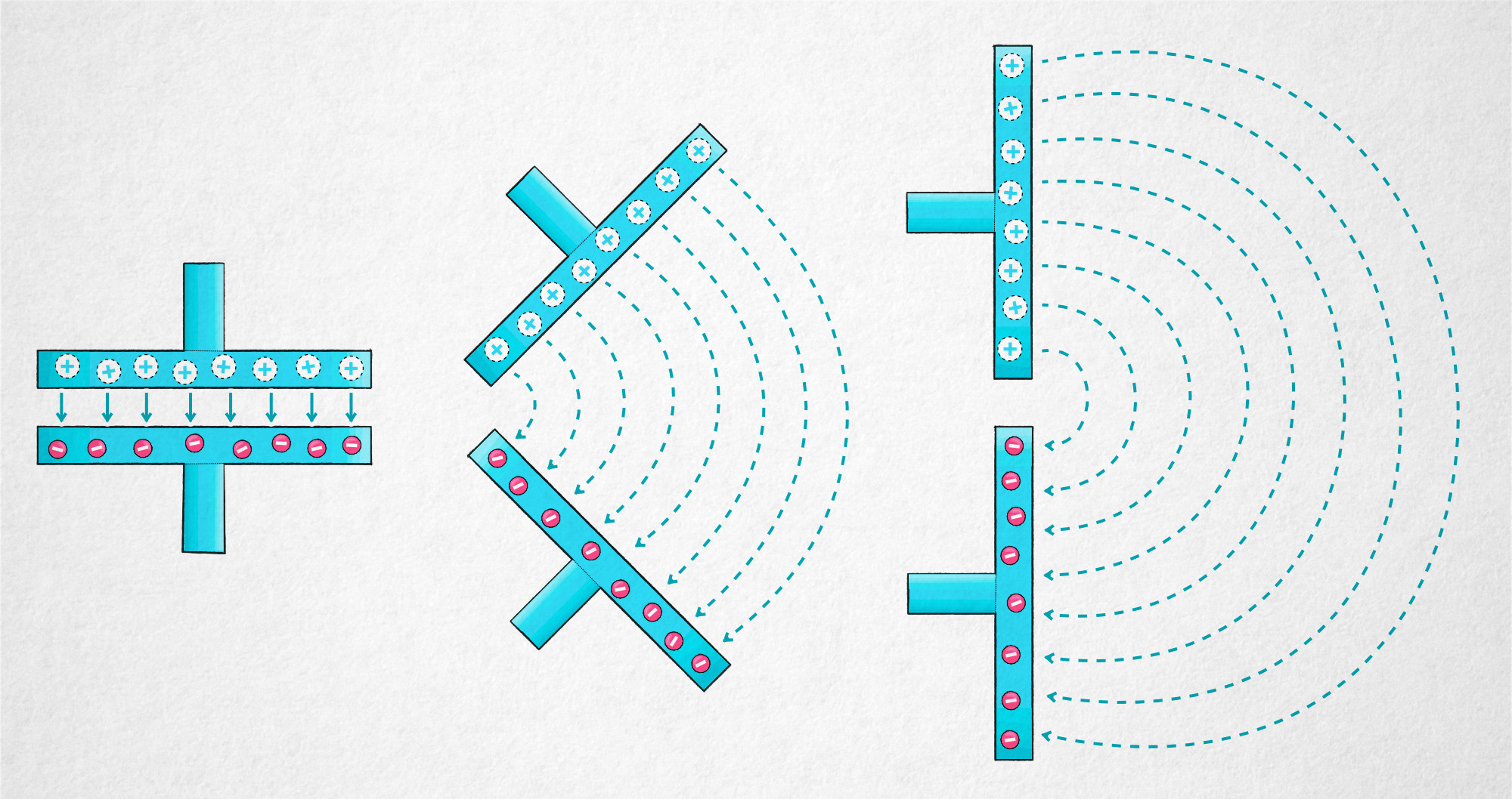
Electric fields can be visualized by plotting the paths of hypothetical positively-charged particles placed in the vicinity. For our ex-capacitor, we’d be seeing arc-shaped lines that connect the plates — and strictly speaking, extend on both sides all the way to infinity.

An unchanging electric field isn’t very useful: if it’s just sitting there for all eternity, it doesn’t convey information nor perform meaningful work. If we push a charge against the direction of the field and then let it loose, the particle will fly away – but that’s just a matter of getting back the energy we expended on pushing it into position in the first place.

The situation changes if we start moving charges back and forth between the plates. This produces an interesting effect: a ripple-like pattern of alternating fields that are getting away from the ex-capacitor at the speed of light:

Field pattern around a simple antenna.

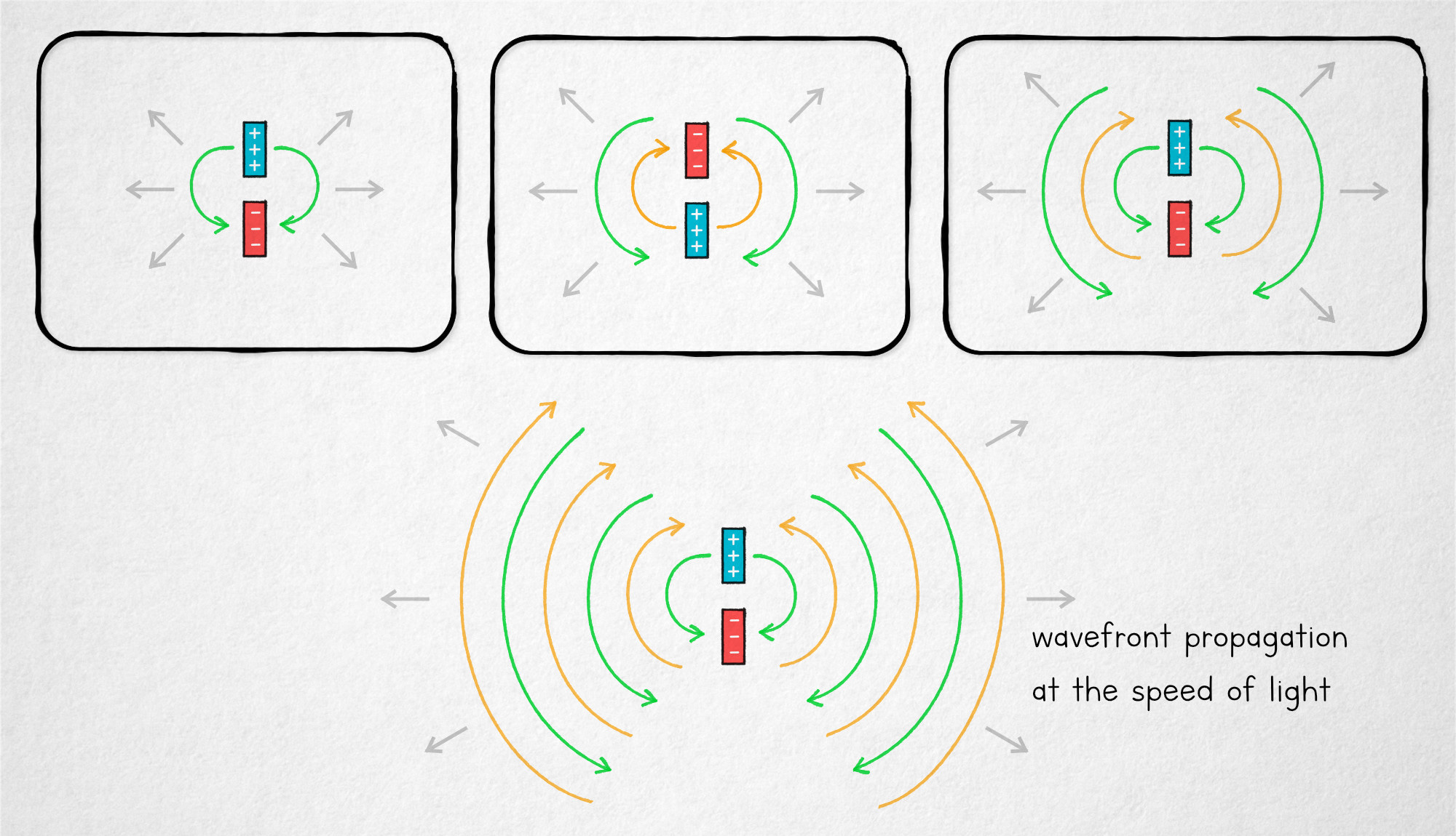
The color corresponds to the direction of the field - i.e., the pull that a charged particle would experience if placed in the vicinity; let’s say that green stands for a “downward” field where the upper half of the antenna is positive and the lower half is negative; yellow is the other way round.

Each transition sneaks away with some amount of energy; on the account of relativity, we can no longer recover this energy directly, but it can be transferred to downstream charges that begin to move back and forth as they “swim” through the gradients of the field; this motion might induce currents in a receiving antenna placed some distance away. It should be fairly evident that the amount of radiated energy must increase not only with the amount of charges shuttled back and forth between the plates, but also with the number of transitions per second – i.e., with the signal’s frequency.

A perfectly uniform waveform is still not useful for communications, but we can encode information by slightly altering the wave’s characteristics — for example, tweaking its amplitude. And if we do it this way, then owing to a clever trick we’ll discuss a bit later, simultaneous transmissions on different frequencies can be told apart on the receiving end.

But first, it’s time for a reality check: if we go back to our dismantled capacitor and hook it up to a signal source, it won’t actually do squat. When we pulled the plates apart, we greatly reduced the device’s capacitance, so we’re essentially looking at an open circuit; a pretty high voltage would be needed to shuffle a decent number of electrons back and forth. Without this motion — i.e., without a healthy current — the radiated energy is negligible.

The most elegant solution to this problem is known as a half-wavelength (“half-wave”) dipole antenna: two rods along a common axis, driven by a sinusoidal signal fed at the center, each rod exactly ¼ wavelength long. If you’re scratching your head, the conversion from frequency (f, in Hz) to wavelength (λ) is:

\(\lambda = \frac{c}{f}\)

The third value — c — is the speed of light per second in your preferred unit of length.

The half-wave dipole has an interesting property: if we take signal propagation delays into account, we can see that every peak of the driving signal reaches the ends of the respective λ/4 rod in a way that adds constructively to the reflection that’s coming back from the high-impedance end:

Resonance of a half-dipole antenna.

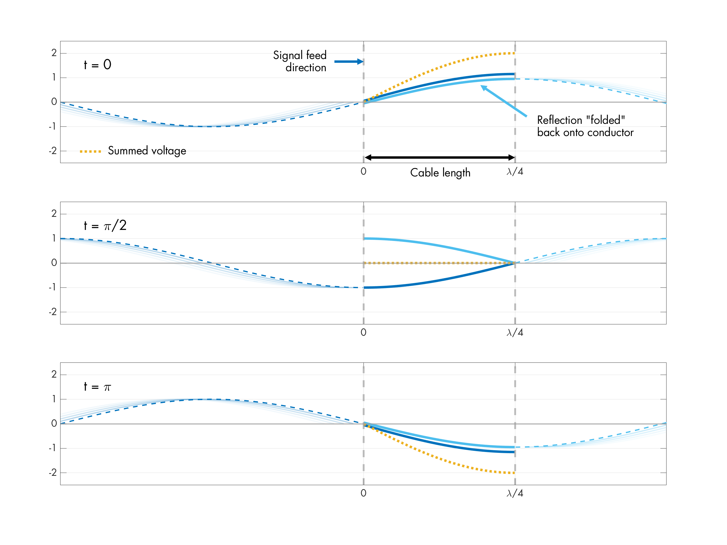
Each reflection is basically just the previous quarter-wave “folded back” onto each rod. (If you’re iffy on signal reflections, I recommend reviewing this article.)

The following animation shows the pattern of superimposed signal and reflections within a single rod. The actual span of the rod is marked by vertical lines. The light blue line is the reflection, which is mirrored back onto the rod. The orange line corresponds to the summed voltage:

The following animation shows both elements of a dipole antenna in action, this time with some modest reflection losses baked in,:

Note the large (36 V) swing at the far ends of the antenna as a result of a far more modest (4 V) swing at the feed point. This makes the antenna efficient and easy to drive.

All dipoles made for odd multiples of half-wavelength (3/2 λ, 5/2 λ, …) exhibit this resonant behavior. Similar resonance is also present at even multiples (1 λ, 2 λ, …), but the standing wave ends up sitting in the wrong spot — constantly getting in the way of driving the antenna rather than aiding the task.

Other antenna lengths are not perfectly resonant, although they might be close enough. An antenna that’s way too short to resonate properly can be improved with an in-line inductor, which adds some current lag. You might have seen antennas with spring-like sections at the base; the practice called electrical lengthening. It doesn’t make a stubby antenna perform as well as a the real deal, but it helps keep the input impedance in check.

Now that we’re have a general grasp of half-wave dipoles, let’s have a look at the animation of actual electric field around a half-wave antenna:

Note the two dead zones along the axis of the antenna; this is due to destructive interference of the electric fields in this axis.

Next, let’s consider what would happen if we placed an identical receiving antenna some distance away from the transmitter. Have a look at receiver A on the right:

Some receiver antenna scenarios.

It’s easy to see that the red dipole is “swimming” through a coherent pattern alternating electric fields: the blue region is pulling electrons toward the upper plate, and yellow pushing them down. The antenna experiences back-and-forth currents between its poles at the transmitter’s working frequency. Further, if the antenna’s length is chosen right, there should be constructive interference of the induced currents too, eventually resulting in much higher signal amplitudes.

The illustration also offers an intuitive explanation of something I didn’t mention before: that dipoles longer than ½ wavelength are more directional. If you look at receiver B on the left, it’s clear that even a minor tilt of a long dipole results in the ends being exposed to opposing electric fields, yielding little or no net current flow.

Not all antennas are dipoles, but most operate in a similar way. Monopoles are just a minor riff on the theme, trading one half of the antenna for a connection to the ground. More complex shapes usually crop up as a way to maintain resonance at multiple frequencies or to fine-tune directionality. You might also bump into antenna arrays; these devices exploit patterns of constructive and destructive interference between digitally-controlled signals to flexibly focus on a particular spot.

The ups and downs of signal modulation

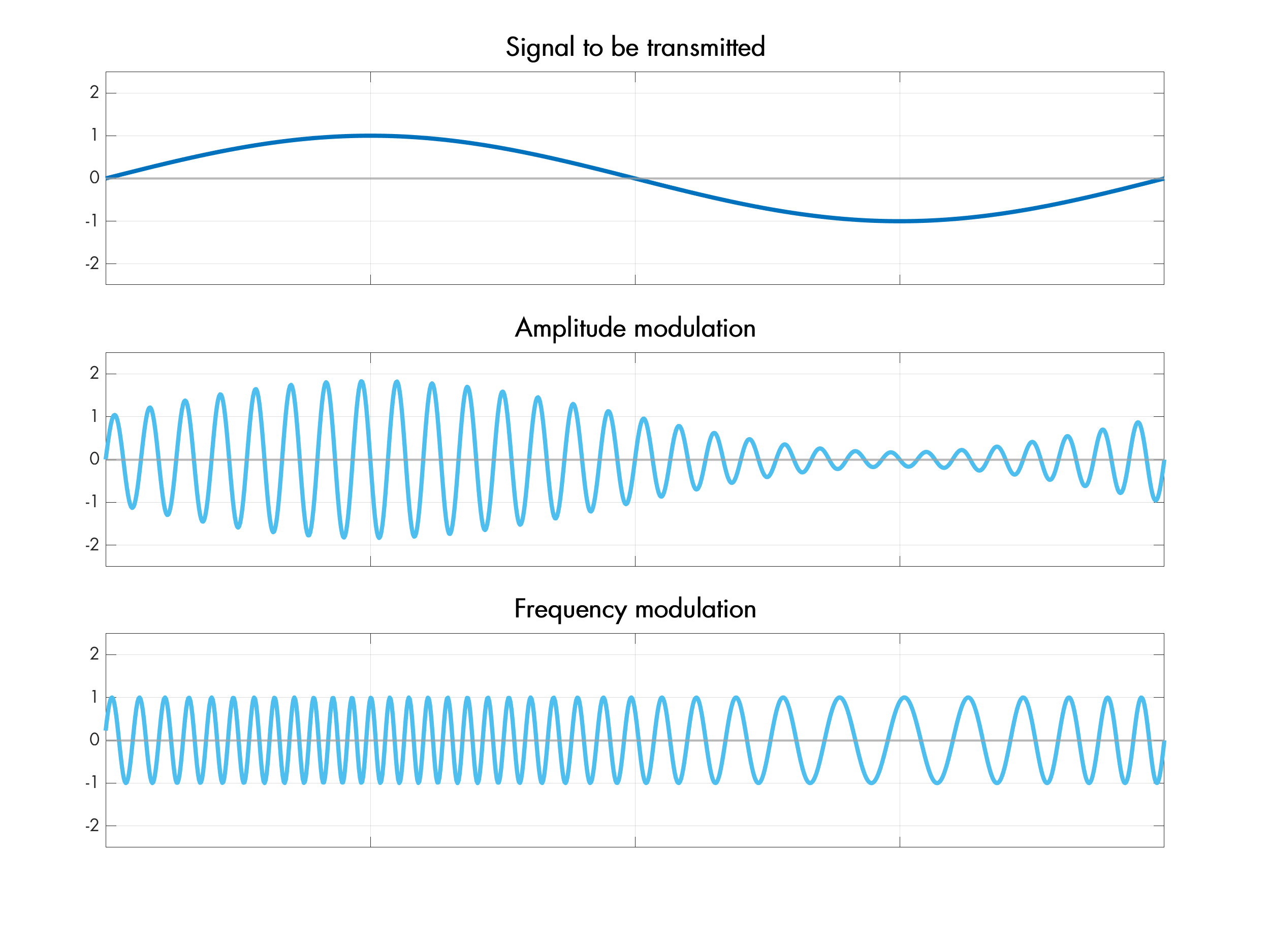
Compared to antenna design, signal modulation is a piece of cake. There’s amplitude modulation (AM), which changes the carrier’s amplitude to encode information; there’s frequency modulation (FM), which shifts the carrier up and down; and there’s phase modulation (PM) — well, you get the drift. We also have quadrature amplitude modulation (QAM), which robustly conveys information via the relative amplitude of two signals with phases offset by 90°.

In any case, once the carrier signal is isolated, demodulation is typically pretty easy to figure out. For AM, the process can be as simple as rectifying the amplified sine wave with a diode, and then running it through a lowpass filter to obtain the audio-frequency envelope. Other modulations are a bit more involved — FM and PM benefit from phase-locked loops to detect shifts — but most of it isn’t rocket surgery.

Still, there are two finer points to bring up about modulation. First, the rate of change of the carrier signal must be much lower than its running frequency. If the modulation is too rapid, you end up obliterating the carrier wave and turning it into wideband noise. The only reason why resonant antennas and conventional radio tuning circuits work at all is that almost nothing changes cycle-to-cycle — so in the local view, you’re dealing with a nearly-perfect, constant-frequency sine.

The other point is that counterintuitively, all modulation is frequency modulation. Intuitively, AM might feel like a clever zero-bandwidth hack: after all, we’re just changing the amplitude of a fixed-frequency sine wave, so what’s stopping us from putting any number of AM transmissions a fraction of a hertz apart?

Well, no dice: recall from the discussion of the Fourier transform that any deviation from a steady sine introduces momentary artifacts in the frequency domain. The scale of the artifacts is proportional to the rate of change; AM is not special and takes up frequency bandwidth too. To illustrate, here’s a capture of a local AM station; we see audio modulation artifacts spanning multiple kHz on both sides of the carrier frequency:

The talk of the town.

Indeed, all types of modulation boil down to taking a low-frequency signal band — such as audio — and transposing it in one way or another to a similarly-sized slice of the spectrum in the vicinity of some chosen center frequency.

At this point, some readers might object: the Fourier transform surely isn’t the only way to think about the frequency spectrum; just because we see halos on an FFT plot, it doesn’t mean they’re really real. In an epistemological sense, this might be right. But as it happens, radio receivers work by doing something that walks and quacks a lot like Fourier…

Inside a superheterodyne receiver

As foreshadowed just moments ago, the basic operation of almost every radio receiver boils down to mixing (multiplying) the amplified antenna signal with a sine wave of a chosen frequency. This is eerily similar to how Fourier-adjacent transforms deconstruct complex signals into individual frequency components.

From the discussion of the discrete cosine transform (DCT) in the earlier article, you might remember that if a matching frequency is present in the input signal, the multiplication yields a waveform with a DC bias proportional to the magnitude of that frequency component. For all other input frequencies, the resulting waveforms average out to zero, if analyzed on a sufficiently long timescale.

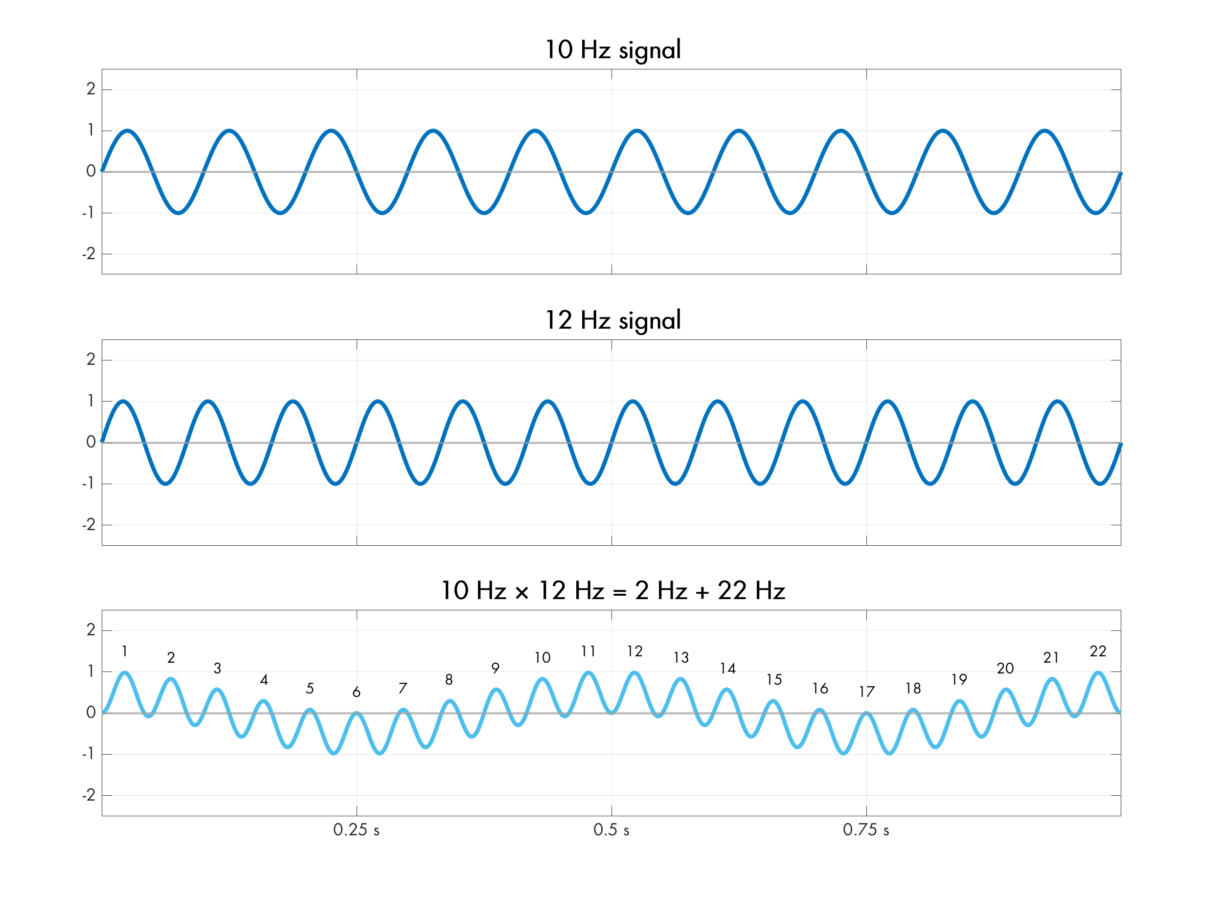
But that averaging timescale is of interest too: in the aforementioned article, we informally noted that the resulting composite waveforms have shorter periods if the original frequencies are far apart, and longer periods if the frequencies are close. Well, as it turns out, for scalar multiplication, the low-frequency cycle is always |f₁ - f₂|, superimposed on top of a (less interesting) high-frequency component f₁ + f₂:

Dropping some sick beats.

This behavior might seem puzzling, but it arises organically from the properties of sine waves. Let’s start with the semi-well-known angle sum identity, which has a cute and easy proof involving triangles:

Cosine angle sum identity. By author.

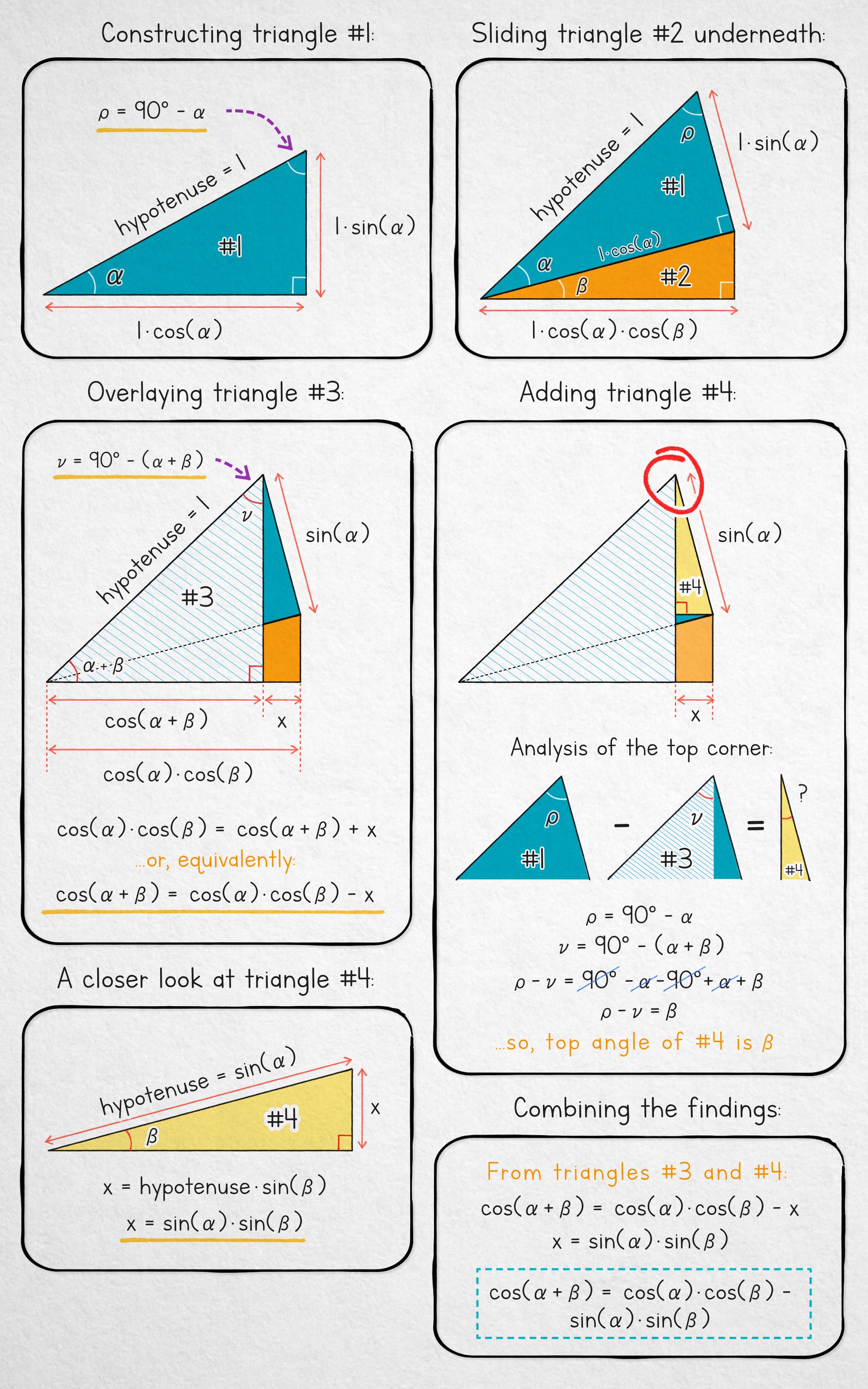
We start with two given angles, α and β. Panel 1 (top left): we construct a right-angle triangle (#1), which has an angle of α and a hypotenuse equal to 1. Next, we calculate the length of the adjacent of that triangle using basic trigonometry — 1 × cos(α). Panel 2 (top right): we slide a second triangle underneath #1. The new triangle (#2) has an angle of β and a hypotenuse of the same length as the adjacent of triangle #1: cos(α); this makes the adjacent of #2 equal to cos(α) × cos(β).

Panel 3 (middle left): we add triangle #3, placing it on top of the other triangles. The new triangle inherits a hypotenuse of 1 from triangle #1, and has a combined angle of α+β as a consequence of being partly inscribed inside #1 and #2. It follows that its adjacent is 1 × cos(α + β).

The bottom edge of the combined figure has a length equal to the known adjacent of #2: cos(α) × cos(β). Alternatively, the length can be expressed as the adjacent of #3 – cos(α + β) – plus some unknown segment, x.

We solve for that mystery segment by looking a new helper triangle (#4). Panel 4 (middle right): we find the top angle of that triangle, which works out to β. Panel 5 (bottom): a quick analysis shows that x is equal to sin(α) × sin(β). Putting it all together, we obtain the following angle sum identity:

\(cos(\alpha + \beta) = cos(\alpha) \cdot cos(\beta) - sin(\alpha) \cdot sin(\beta)\)

Now that we have this expansion for cos(α + β), we can trivially extend it to cos(α - β):

\(\begin{array}{c} cos(a - b) = cos(a + (-b)) \\ = cos(a)\cdot cos(-b) - sin(a) \cdot sin(-b) \\ \\ \textrm{Self-evident trigonometric substitutions:} \\ cos(-b) = cos(b) \\ sin(-b) = -sin(b) \\ \\ \textrm{Formula after substitutions:} \\ cos(a - b) = cos(a) \cdot cos(b) + sin(a) \cdot sin(b) \end{array}\)

Together, the equations for cos(α + β) and cos(α – β) let us show that:

\(\begin{array}{c} cos(a - b) - cos(a+b)\\ = \cancel{cos(a) \cdot cos(b)} + sin(a) \cdot sin(b) \\ - \cancel{cos(a) \cdot cos(b)} + sin(a) \cdot sin(b) \\ = 2 \cdot sin(a) \cdot sin(b) \end{array}\)

If we divide both sides by two and flip the expression around, we end up with a formula that equates the product of two sine frequencies to an average of two independent cosines running at |f₁ - f₂| and f₁ + f₂:

\(sin(a) \cdot sin(b) = \frac{cos(a - b) - cos(a + b)}{2}\)

Heck, we don’t even need to believe in trigonometry. A closely-related phenomenon has been known to musicians for ages: when you simultaneously play two very similar tones, you end up with an unexpected, slowly-pulsating “beat frequency”. Here’s a demonstration of a 5 Hz beat produced by combining 400 Hz and 405 Hz:

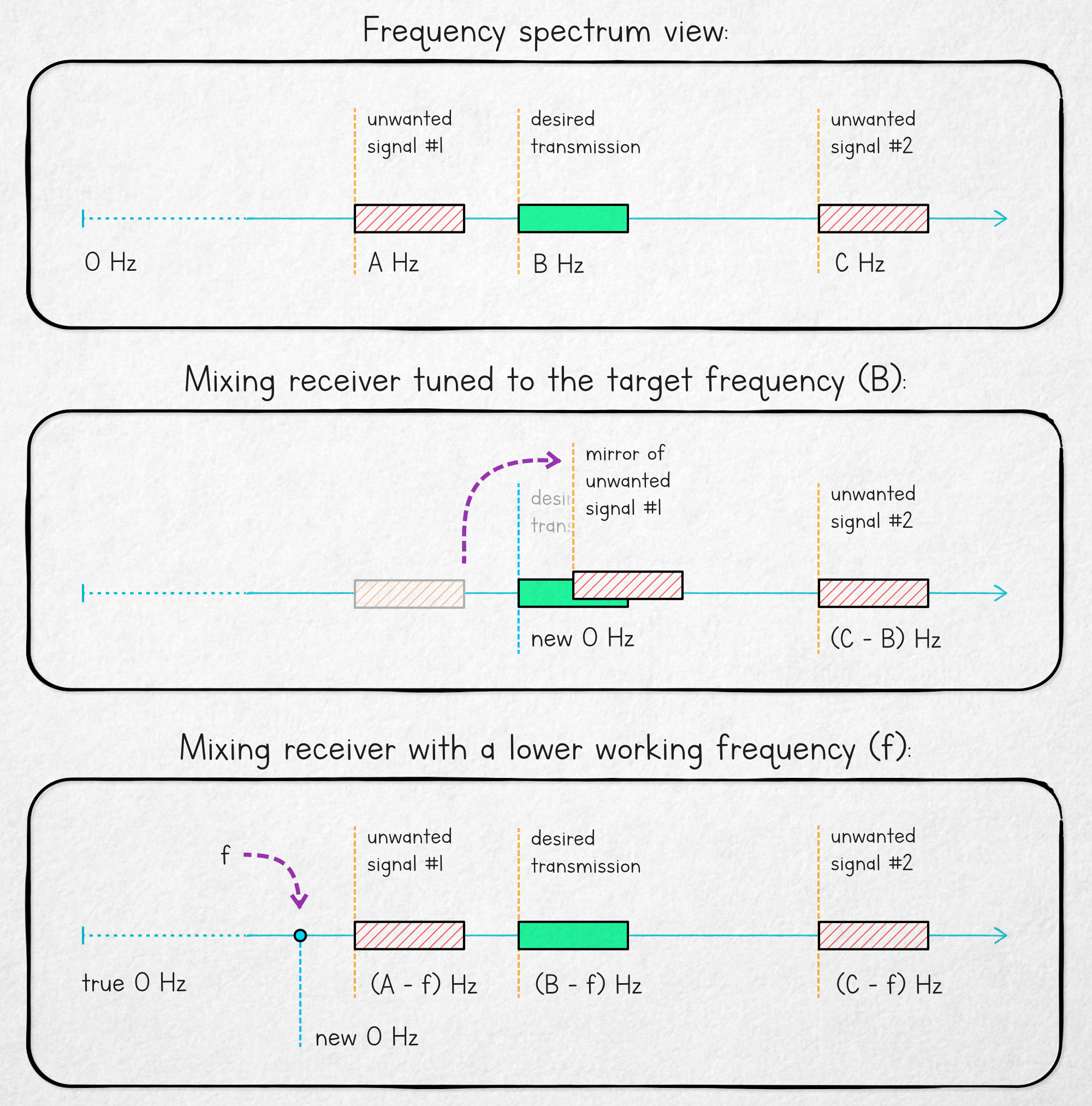
In any case, back to radio: it follows that if one wanted to receive transmissions centered around 10 MHz, a straightforward approach would be to mix the input RF signal with a 10 MHz sine. According to our formulas, this should put the 10.00 MHz signal at DC, downconvert 10.01 MHz to a 10 kHz beat (with an extra 20.01 MHz component), turn 10.02 MHz into 20 kHz (+ 20.02 MHz), and so forth. With the mixing done, the next step would be to apply a lowpass filter to the output, keeping only the low frequencies that are a part of the modulation scheme - and getting rid of everything else, including the unwanted f₁ + f₂ components.

The folly of this method is the modulo operator in the |f₁ - f₂| formula, a consequence of cos(x) being the same as cos(-x). This causes beat frequencies to exhibit symmetry around 0 Hz on the output side. In other words, in the aforementioned 10 MHz example, the input component at 9.99 MHz produces an image at 10 kHz too — precisely where 10.01 MHz was supposed to go. To avoid this mirroring, receivers mix the RF input with a frequency lower than the signal of interest, shifting it to a constant non-zero intermediate frequency (IF) — and then using bandpass filters to pluck out the relevant bits.

In this design — devised by Edwin Armstrong around 1919 and dubbed superheterodyne — the fundamental mirroring behavior is still present, but the point of symmetry can be placed far away. With this trick up our sleeve, accidental mirror images of unrelated transmissions become easier to manage — for example, by designing the antenna to have a narrow frequency response and not pick up the offending signals at all, or by putting an RF lowpass filter in front of the mixer. The behavior of superheterodynes is sometimes taken into account for radio spectrum allocation purposes, too.

👉 For a thematic catalog of articles on electronics, click here.

---

I write well-researched, original articles about geek culture, electronic circuit design, and more. If you like the content, please subscribe. It’s increasingly difficult to stay in touch with readers via social media; my typical post on X is shown to less than 5% of my followers and gets a ~0.2% clickthrough rate.